วิธีจับคู่สองคอลัมน์ใน Excel

คู่มือฉบับสมบูรณ์เพื่อเปรียบเทียบสองคอลัมน์ใน Excel และรับข้อมูลที่ตรงกันหรือความแตกต่าง ไฮไลต์หรือดึงข้อมูล

เมื่อคุณทำงานกับข้อมูลใน Excel คุณอาจต้องเปรียบเทียบคอลัมน์เพื่อค้นหาความเหมือนและความแตกต่างระหว่างข้อมูล การเปรียบเทียบคอลัมน์มีประโยชน์มากสำหรับการจัดระเบียบและวิเคราะห์ข้อมูล การเปรียบเทียบข้อมูลจากสองคอลัมน์ด้วยตนเองอาจเป็นงานที่ต้องใช้เวลามากและต้องใช้ความพยายามมาก คุณจึงสามารถใช้สูตร Excel ต่างๆ เพื่อจับคู่คอลัมน์ได้

Excel มีวิธีการและฟังก์ชันที่หลากหลายสำหรับการเปรียบเทียบคอลัมน์และการค้นหาข้อมูลที่ตรงกันและไม่ตรงกัน. คุณสามารถใช้ตัวดำเนินการเชิงตรรกะ เช่น VLOOKUP, MATCH, AND, INDEX, IF, COUNTIF, ISERROR, IFERROR – หรือ Conditional Formatting rule เพื่อเปรียบเทียบและจับคู่ข้อมูล ในบทความนี้ เราจะพูดถึงวิธีการต่างๆ ในการเปรียบเทียบคอลัมน์ใน Excel สำหรับการจับคู่และความแตกต่าง

การเปรียบเทียบสองคอลัมน์ทีละแถวสำหรับการจับคู่หรือความแตกต่าง

วิธีที่ง่ายที่สุดในการเปรียบเทียบสองคอลัมน์ ใน Excel เป็นการเปรียบเทียบแบบแถวต่อแถวแบบบรรทัดต่อบรรทัดอย่างง่าย วิธีนี้จะตรวจสอบว่าค่าในคอลัมน์หนึ่งตรงกับค่าในอีกคอลัมน์หนึ่งในแถวเดียวกันหรือไม่ โดยจะเปรียบเทียบเฉพาะค่าในแถวเดียวกัน ไม่ใช่ชุดข้อมูลทั้งหมด มีสูตรหลายประเภทที่คุณสามารถใช้เพื่อเปรียบเทียบสองคอลัมน์ทีละแถว โดยใช้ตัวดำเนินการเปรียบเทียบอย่างง่าย ฟังก์ชัน IF และฟังก์ชัน EXACT

เปรียบเทียบคอลัมน์โดยใช้ตัวดำเนินการเท่ากับ

วิธีที่ง่ายที่สุดในการเปรียบเทียบข้อมูลของสองคอลัมน์ทีละแถวเพื่อค้นหาการจับคู่คือการใช้ตัวดำเนินการเปรียบเทียบ ด้วย’เท่ากับ'(=) คุณสามารถเปรียบเทียบเซลล์ในสองคอลัมน์สำหรับการจับคู่และรับผลลัพธ์ว่าจริงหรือเท็จ

ตัวอย่างที่ 1:

ตัวอย่างเช่น เราจะเปรียบเทียบสองคอลัมน์ (ครบกำหนดเรียกเก็บเงินและเรียกเก็บเงินในภาพหน้าจอด้านล่าง) เพื่อดูว่าตรงกันหรือไม่ ในการทำเช่นนั้น เราจะใช้สูตรง่ายๆ ด้านล่าง:

=B2=C2

ค่าใน B2 ตรงกับค่าใน C2 ดังนั้นสูตรจะคืนค่าเป็น TRUE ขั้นแรก ให้ป้อนสูตรในเซลล์ D2 แล้วคัดลอกลงในเซลล์อื่นโดยลากจุดจับเติมเพื่อเปรียบเทียบคอลัมน์ B และ C ทีละแถว จุดจับเติมเป็นสี่เหลี่ยมสีเขียวขนาดเล็กที่มุมล่างขวาของเซลล์ที่เลือก

เมื่อคุณลาก เติมที่จับจากเซลล์ D2 ถึง D12 เคอร์เซอร์จะเปลี่ยนเป็นเครื่องหมายบวกสีดำ

ในขณะที่คุณใช้ สูตรผ่านเซลล์ D2 ถึง D12 จะเปรียบเทียบค่าทีละแถว และคุณจะเห็นบางแถวตรงกันในขณะที่บางแถวไม่ตรงกัน ตัวอย่างเช่น ค่าจากเซลล์ B4 ไม่ตรงกับเซลล์ C4 ที่อยู่ติดกัน ดังนั้นค่าในเซลล์ D4 จึงเป็น FALSE

ตัวอย่างที่ 2:

เราได้เห็นแล้วว่าสูตรข้างต้นจัดการกับตัวเลขอย่างไร แต่ยังเปรียบเทียบวันที่ เวลา และสตริงข้อความได้เป็นอย่างดีอีกด้วย ให้เราดูว่าสูตรเปรียบเทียบคอลัมน์กับค่าข้อความอย่างไร

=A2=B2

สูตรจะค้นหาการจับคู่ที่ถูกต้องระหว่างสองคอลัมน์ และจะไม่พลาดแม้แต่อักขระเว้นวรรคแม้แต่ตัวเดียว จากนั้นจะคืนค่า TRUE หากตรงตามเงื่อนไขหรือคืนค่า FALSE ที่อยู่สำหรับการเรียกเก็บเงินในเซลล์ A2 ตรงกับที่อยู่ในการจัดส่งในเซลล์ B2 ดังนั้นเราจึงได้รับ TRUE นอกจากนี้ ที่อยู่ในเซลล์ A5 ไม่ตรงกับที่อยู่ในเซลล์ B5 – อักขระตัวสุดท้ายจะแตกต่างกันในเซลล์ B5 ดังนั้นจึงคืนค่าเป็น FALSE

เปรียบเทียบคอลัมน์โดยใช้ฟังก์ชัน IF

อีกวิธีหนึ่งที่เราสามารถทำได้ เปรียบเทียบสองคอลัมน์ทีละแถวโดยใช้ฟังก์ชัน IF ฟังก์ชัน IF จะตรวจสอบว่าตรงตามเงื่อนไขหรือเกณฑ์และส่งกลับค่าที่ระบุหนึ่งค่าหากเงื่อนไขเป็น TRUE หรือค่าอื่นหากเงื่อนไขเป็น FALSE แม้ว่าวิธีนี้จะคล้ายกับวิธีการข้างต้น แต่เราสามารถใช้เพื่อให้ได้ผลลัพธ์เชิงพรรณนามากกว่าแค่ TRUE หรือ FALSE

ตัวอย่างเช่น เราสามารถใช้สูตรด้านล่างเพื่อเปรียบเทียบสองคอลัมน์และหากมี ตรงกัน เราจะได้ผลลัพธ์”จ่าย”หรือ”ไม่จ่าย”หากไม่มีการจับคู่:

=IF(B2=C2,”Paid”,”Not Paid”)

ในสูตรข้างต้น ฟังก์ชัน IF ตรวจสอบว่าค่าใน B2 เท่ากับค่าใน C2 หรือไม่ และหากเงื่อนไขเป็น True จะส่งกลับข้อความว่า”ชำระแล้ว”หากเงื่อนไขเป็นเท็จ จะส่งกลับ”ไม่ชำระเงิน”จำนวนเงินที่ครบกำหนดชำระใน B2 และจำนวนเงินที่ชำระใน C2 จะเท่ากัน ดังนั้นจึงส่งคืน”ชำระแล้ว”ใน D2 แต่จำนวนเงินใน B5 และ C5 ไม่ตรงกัน ดังนั้นสูตรจะแสดงผลว่า”ไม่ชำระเงิน”ใน D5

สำหรับการจับคู่เท่านั้น:

ในกรณีที่คุณต้องการค้นหาเฉพาะรายการที่ตรงกันในสองคอลัมน์ คุณสามารถใช้สูตรด้านล่าง:

=IF(B2=C2,”Paid”,””)

สูตรข้างต้นจะตรวจสอบว่าค่าในคอลัมน์ B เท่ากับค่าในคอลัมน์ C หรือไม่ ทีละแถว หากเงื่อนไขเป็นจริง เราจะได้รับสตริงข้อความ”ชำระเงิน”และหากเงื่อนไขเป็นเท็จ เราจะไม่ได้รับอะไรเลย (สตริงว่าง)

สำหรับส่วนต่างเท่านั้น:

หากต้องการค้นหาเซลล์ที่มีค่าต่างกันในแถวเดียวกัน ให้ลองใช้สูตรด้านล่าง:

=IF( B4<>C4,”Not Paid”,””)

สูตรข้างต้นตรวจสอบว่าค่าในคอลัมน์ B ไม่เท่ากับค่าในคอลัมน์ C หรือไม่ ทีละแถว หากเงื่อนไขเป็นจริง เราจะได้รับสตริงข้อความ”ไม่ชำระเงิน”และหากเงื่อนไขเป็นเท็จ เราจะไม่ได้รับอะไรเลย (สตริงว่าง)

หมายเหตุ: สูตรเท่ากับสูตรและฟังก์ชัน IF ไม่คำนึงถึงขนาดตัวพิมพ์ ซึ่งหมายความว่าจะละเว้นกรณีเมื่อเปรียบเทียบค่าข้อความ

เปรียบเทียบ สองคอลัมน์สำหรับการจับคู่แบบตรงตามตัวพิมพ์เล็กและใหญ่ในแถวเดียวกันโดยใช้ฟังก์ชัน EXACT

สูตรข้างต้นจะไม่สนใจกรณีเมื่อเปรียบเทียบค่าข้อความ หากคุณต้องการเปรียบเทียบตัวพิมพ์เล็กและตัวพิมพ์ใหญ่ คุณต้องใช้ฟังก์ชัน EXACT ฟังก์ชัน Excel EXACT ใช้เพื่อเปรียบเทียบสตริงข้อความสองสตริงและคืนค่า TRUE หากค่าทั้งสองมีค่าเท่ากัน มิฉะนั้นจะเป็น FALSE คุณสามารถใช้ EXACT อย่างเดียวหรือใช้ฟังก์ชัน IF ก็ได้ (ในกรณีที่คุณต้องการได้ผลลัพธ์เชิงพรรณนาแทนที่จะเป็นเพียง TRUE หรือ FALSE

ตัวอย่างเช่น ลองเปรียบเทียบรายชื่อบริษัทจากฐานข้อมูลต่างๆ แล้วดูว่า เป็นการจับคู่แบบตรงทั้งหมดโดยใช้ฟังก์ชัน EXACT แบบธรรมดา:

=EXACT(A2,B2)

สูตรด้านบนจะตรวจสอบว่าสตริงข้อความจาก A2 และ B2 เป็นการจับคู่แบบตรงตามตัวพิมพ์เล็กและตัวพิมพ์ใหญ่ จากนั้น จะคืนค่า FALSE เนื่องจาก คำว่า “St” ใน A2 เป็นตัวพิมพ์เล็กในขณะที่ B2 เป็นตัวพิมพ์ใหญ่

ในกรณีที่คุณต้องการ เพื่อให้ได้ผลลัพธ์เชิงพรรณนา คุณต้องใช้ฟังก์ชัน IF กับฟังก์ชัน EXACT:

=IF(EXACT(A3,B3),”Match”,”Check Database”)

ในสูตรข้างต้น ค่า EXACT ฟังก์ชันจะตรวจสอบว่าค่าในเซลล์ A3 และ B3 ตรงกันทุกประการหรือไม่ อย่างไรก็ตาม คำแรก’ANGELO’จะใช้ตัวพิมพ์ใหญ่ใน B2 ซึ่งแตกต่างจากชื่อบริษัทใน A2 ดังนั้นฟังก์ชัน EXACT จะส่งกลับ FALSE ดังนั้น ฟังก์ชัน IF จะส่งกลับสตริงข้อความ”ตรวจสอบฐานข้อมูล”สำหรับเอาต์พุต FALSE

ในแถวที่ 5 ค่าของเซลล์ A5 และ B5 เป็นการจับคู่แบบคำนึงถึงขนาดตัวพิมพ์ ดังนั้น ฟังก์ชัน IF จะได้รับผลลัพธ์ TRUE จากฟังก์ชัน EXACT และส่งกลับ”MATCH”แทนค่า

เปรียบเทียบสองคอลัมน์ถ้ามากกว่าหรือน้อยกว่า

h2>

บางครั้ง คุณอาจต้องการเปรียบเทียบคอลัมน์และตรวจสอบว่าค่าในคอลัมน์หนึ่งมากกว่าหรือน้อยกว่าคอลัมน์อื่นๆ ตัวอย่างเช่น หากคุณมีวันที่สองคอลัมน์และต้องการเปรียบเทียบวันที่ที่อยู่ภายหลังในแถวเดียวกัน (อาจเปรียบเทียบวันหมดอายุของผลิตภัณฑ์) คุณสามารถใช้การดำเนินการทางตรรกะอย่างง่ายเพื่อค้นหาได้

หากต้องการทราบว่าผลิตภัณฑ์หมดอายุหรือไม่ ให้เปรียบเทียบสองคอลัมน์ว่าคอลัมน์ C มากกว่าคอลัมน์ B:

=IF(C2>B2,”Yes”,”No”)

สูตรข้างต้น ตรวจสอบว่าค่าในเซลล์ C2 มากกว่าเซลล์ B2 หรือไม่ หากเป็น TRUE ฟังก์ชัน IF จะส่งกลับ’Yes’มิฉะนั้น’No’

เปรียบเทียบหลายคอลัมน์ ทีละแถวสำหรับการจับคู่

เราได้เห็นวิธีเปรียบเทียบสองคอลัมน์ทีละแถวแล้ว แต่คุณยังสามารถเปรียบเทียบหลายคอลัมน์สำหรับรายการที่ตรงกันในแถวเดียวกันได้ มีสองวิธีที่คุณสามารถเปรียบเทียบหลายคอลัมน์ได้-ค้นหารายการที่ตรงกันภายในเซลล์ทั้งหมดในแถวเดียวกันหรือค้นหาที่ตรงกันในสองเซลล์ในแถวเดียวกัน

ค้นหารายการที่ตรงกันในเซลล์ทั้งหมดภายในแถวเดียวกัน

วิธีที่ 1: หากคุณมีชุดข้อมูลที่มีมากกว่าสองคอลัมน์ (หลายคอลัมน์) และคุณต้องการค้นหาแถวที่มีค่าเดียวกันในทุกคอลัมน์ คุณสามารถทำเช่นนี้ได้ด้วยฟังก์ชัน IF และ AND:

=IF(AND(A3=B3,A3=C3),”All Match”,””)

ฟังก์ชัน AND จะทดสอบหลายเงื่อนไขพร้อมกัน (A3=B3 และ A3=C3) และคืนค่า TRUE ก็ต่อเมื่ออาร์กิวเมนต์ทั้งหมดประเมินเป็น TRUE ฟังก์ชัน AND จะคืนค่า FALSE แม้ว่าหนึ่งในอาร์กิวเมนต์จะประเมินเป็น FALSE คุณสามารถเพิ่มหลายเงื่อนไขในฟังก์ชัน AND ได้โดยการใส่เครื่องหมายจุลภาคระหว่างแต่ละเงื่อนไข

ดังที่คุณเห็นด้านล่าง ฟังก์ชัน AND จะคืนค่าเป็น จริง หากเซลล์ทั้งหมดมีค่าเท่ากันในแถวเดียวกัน จากนั้น ฟังก์ชัน IF จะส่งคืนข้อความ”All Match”หากฟังก์ชัน AND คืนค่า TRUE

วิธีที่ 2: หากชุดข้อมูลของคุณมีคอลัมน์จำนวนมาก คุณสามารถใช้ฟังก์ชัน COUNTIF เพื่อทำให้สูตรของคุณกระชับ:

=IF(COUNTIF($A3:$D3, $A3)=4,”ตรงกันทั้งหมด”,””)

โดยที่ 4 หมายถึงจำนวนคอลัมน์ที่คุณกำลังเปรียบเทียบในสูตร ฟังก์ชัน COUNTIF ใช้เพื่อนับตัวเลขที่ตรงตามเกณฑ์ที่กำหนด

สูตร COUNTIF จะตรวจสอบว่าแถวนั้นมีค่าเท่ากันในเซลล์ทั้งหมดหรือไม่ (A3:D3) และส่งกลับจำนวนที่ตรงกันทั้งหมด. และหากคอลัมน์ทั้งหมดตรงกันภายในแถวเดียวกัน (ผลลัพธ์ของฟังก์ชัน COUNTIF) เท่ากับจำนวนคอลัมน์ คุณจะได้รับสตริงข้อความที่ระบุว่า”ตรงกันทั้งหมด”

ค้นหาที่ตรงกันในสองเซลล์ในแถวเดียวกัน

วิธีที่ 1: สมมติว่าคุณมีหลายเซลล์ (3 ) และคุณต้องการค้นหารายการที่ตรงกันในสองคอลัมน์ในแถวเดียวกัน คุณสามารถทำได้โดยใช้ฟังก์ชัน IF และ OR ในการดำเนินการนี้ เราสามารถใช้สูตรด้านล่าง:

=IF(OR(A3=B3, B3=C3, A3=C3),”Match”,””)

ในสูตรข้างต้น ฟังก์ชัน OR เปรียบเทียบแต่ละคอลัมน์กับคอลัมน์อื่นๆ และหากมีคอลัมน์ใดในสองคอลัมน์ขึ้นไปที่มีค่าเดียวกันตรงกันภายในแถวเดียวกัน คอลัมน์นั้นจะคืนค่า TRUE ฟังก์ชัน IF จะส่งคืนข้อความ’Match’เมื่อได้รับค่า TRUE จากฟังก์ชัน OR

วิธีที่ 2: หากคุณมีคอลัมน์จำนวนมากเกินไปที่จะเปรียบเทียบ สูตร OR ด้านบนอาจใหญ่และซับซ้อนเกินไป เพื่อหลีกเลี่ยงปัญหานี้ คุณสามารถเพิ่มฟังก์ชัน COUNTIF ได้หลายฟังก์ชัน:

=IF(COUNTIF(B3:D3,A3)+COUNTIF(C3:D3,B3)+(C3=D3)=0,”Unique”,”ตรงกัน”)

ที่นี่ ฟังก์ชัน COUNTIF แรกจะตรวจสอบและนับจำนวนเซลล์ (คอลัมน์) ที่มีค่าเท่ากับคอลัมน์แรก (A3) และฟังก์ชัน COUNTIF ที่สองจะตรวจสอบจำนวนคอลัมน์ที่มีค่าเท่ากับคอลัมน์ที่สอง และอื่นๆ จากนั้นผลลัพธ์ของฟังก์ชัน COUNTIF ทั้งหมดจะถูกรวมเข้าด้วยกัน ดังนั้น หากจำนวนสุดท้ายเท่ากับ 0 สูตรจะส่งคืนสตริงข้อความ”ไม่ซ้ำ”หากการนับเป็นอย่างอื่นที่ไม่ใช่ 0 เราจะได้รับ’การจับคู่’เป็นผลลัพธ์

เปรียบเทียบและเน้น คอลัมน์ที่ตรงกัน/ไม่ตรงกัน

ถ้าคุณต้องการเปรียบเทียบสองคอลัมน์และเน้นแถวที่มีข้อมูลที่ตรงกันหรือข้อมูลไม่ตรงกันแทนที่จะแสดงผลลัพธ์ในคอลัมน์ที่แยกจากกัน คุณสามารถใช้การจัดรูปแบบตามเงื่อนไขใน Excel ได้ การจัดรูปแบบตามเงื่อนไขเป็นฟีเจอร์ใน Excel ที่สามารถเน้นข้อมูลตามชุดของกฎ ด้วยการจัดรูปแบบตามเงื่อนไข คุณสามารถระบุค่าที่ตรงกันหรือค่าที่แตกต่างกันในสองคอลัมน์ได้อย่างชัดเจน

เปรียบเทียบสองคอลัมน์และไฮไลต์ข้อมูลที่ตรงกันในแถวเดียวกัน (เคียงข้างกัน)

ถ้าคุณต้องการ หากต้องการเปรียบเทียบสองคอลัมน์และไฮไลต์ข้อมูลที่เหมือนกันในแถวเดียวกัน ให้ทำตามขั้นตอนด้านล่าง:

ขั้นแรก ให้เลือกเซลล์ที่คุณต้องการเปรียบเทียบและไฮไลต์ คุณสามารถเลือกคอลัมน์เดียวหรือหลายคอลัมน์ได้หากต้องการเน้นทั้งแถว

ภายใต้’หน้าแรก’คลิกเมนู’การจัดรูปแบบตามเงื่อนไข’ในกลุ่มสไตล์ แล้วเลือกตัวเลือก’กฎใหม่…’จากเมนู

ซึ่งจะเปิดกล่องโต้ตอบกฎการจัดรูปแบบใหม่ ในหน้าต่างข้อความนั้น ให้เลือกประเภทกฎ’ใช้สูตรเพื่อกำหนดเซลล์ที่จะจัดรูปแบบ’

หลัง ที่ พิมพ์สูตรต่อไปนี้ในฟิลด์’จัดรูปแบบค่าที่สูตรนี้เป็นจริง:’:

=$A1=$B1

อย่างที่คุณเห็น นี่เป็นสูตร’เท่ากับ’ง่ายๆ ที่จะตรวจสอบว่า ค่าในเซลล์ A1 เท่ากับ B1 แต่เราได้เพิ่มเครื่องหมาย’$’ก่อนป้ายชื่อคอลัมน์ A และ B เพื่อล็อกคอลัมน์ให้เป็นข้อมูลอ้างอิงแบบสัมบูรณ์ ดังนั้น เฉพาะหมายเลขแถวเท่านั้นที่เปลี่ยนแปลงโดยอัตโนมัติสำหรับแต่ละแถวเมื่อใช้สูตร

ถัดไป คลิกที่ ปุ่ม’รูปแบบ’เพื่อปรับแต่งรูปลักษณ์ที่คุณต้องการสำหรับแถวที่ไฮไลต์

ในหน้าต่างโต้ตอบรูปแบบเซลล์ คุณสามารถเปลี่ยนขนาดแบบอักษร สีแบบอักษร เส้นขอบของเซลล์ รูปแบบตัวเลข ฯลฯ เพื่อเน้นการจับคู่ แถวที่มีสีพื้นหลังต่างกัน สลับไปที่แท็บเติม แล้วเลือกสีจากส่วนสีพื้นหลัง คุณยังสามารถเปลี่ยนสไตล์ลวดลายและสีลวดลายของเซลล์ที่เน้นสีได้อีกด้วย เมื่อคุณเลือกรูปแบบเสร็จแล้ว ให้คลิกปุ่ม’ตกลง’

อีกครั้ง คลิก’ตกลง’ใน กล่องโต้ตอบกฎการจัดรูปแบบใหม่เพื่อใช้การจัดรูปแบบ

เซลล์ที่มีค่าที่ตรงกันในทั้งสองคอลัมน์ A และ B จะ จะถูกเน้นดังที่แสดงด้านล่าง

หากคุณมีข้อมูลที่ตรงกันน้อยกว่าข้อมูลที่ไม่ตรงกันในตาราง คุณสามารถพลิก เงื่อนไขเพื่อเน้นความแตกต่างของข้อมูลระหว่างสองคอลัมน์

ตัวอย่างเช่น เราสามารถใช้กฎการจัดรูปแบบตามเงื่อนไขด้านล่างเพื่อเน้นความแตกต่างระหว่างคอลัมน์ A และ B:

=$A1<>$B1

หรือ

=$A1=$B1=FALSE

ขั้นแรก เลือกชุดข้อมูลและเปิดหน้าต่างกฎการจัดรูปแบบใหม่ ตามที่เราแสดงให้คุณเห็นด้านบน จากนั้นเลือกประเภทกฎ’ใช้สูตรเพื่อกำหนดเซลล์ที่จะจัดรูปแบบ’จากนั้น ป้อนกฎข้อใดข้อหนึ่งข้างต้นแล้วคลิกปุ่ม’รูปแบบ’

ถัดไป เลือกการจัดรูปแบบของคุณ ต้องการสมัครและคลิก’ตกลง’และคลิก’ตกลง’อีกครั้งเพื่อใช้การจัดรูปแบบ

เปรียบเทียบสองคอลัมน์และเน้นค่าที่ซ้ำกัน

หากคุณต้องการเปรียบเทียบสองคอลัมน์และเน้นค่าที่มีอยู่ในทั้งสองคอลัมน์แม้ว่าจะไม่ได้อยู่ในแถวเดียวกัน คุณสามารถใช้กฎการจัดรูปแบบตามเงื่อนไขที่กำหนดไว้ล่วงหน้าหรือกฎการจัดรูปแบบที่กำหนดเองได้

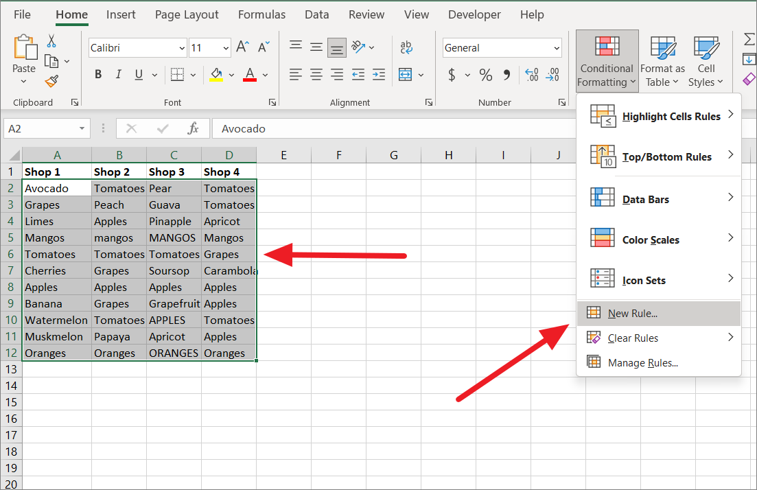
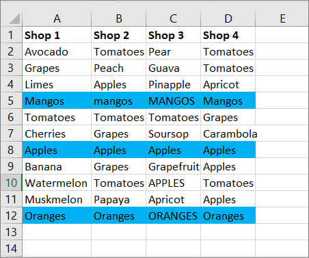
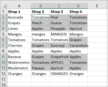
สำหรับ ตัวอย่างเช่น เรามีผลไม้ 2 รายการจากร้านค้าต่างๆ และเราต้องการเน้นผลไม้ที่มีขายในทั้งสองร้าน โดยทำดังนี้:

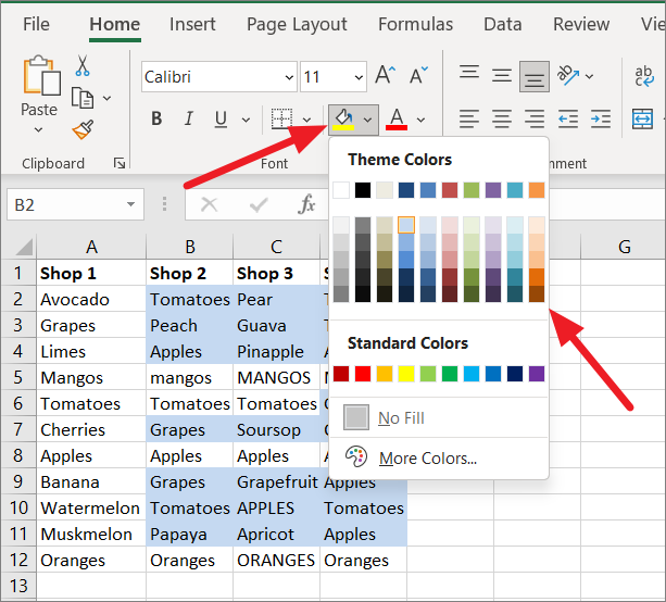
ขั้นแรก เลือกคอลัมน์ที่คุณต้องการเปรียบเทียบ แล้วคลิกเมนู”การจัดรูปแบบตามเงื่อนไข”จากกลุ่มสไตล์

จากนั้น เลื่อนเคอร์เซอร์ไปที่ตัวเลือก’ไฮไลต์กฎของเซลล์’จากเมนูแบบเลื่อนลงและเลือก ตัวเลือก’ค่าที่ซ้ำกัน’

ในกล่องโต้ตอบค่าที่ซ้ำกัน ให้เลือก’ทำซ้ำ’จากดรอปด้านซ้าย-ลง

จากนั้น เลือกรูปแบบจากเมนูแบบเลื่อนลงด้านขวาแล้วคลิก’ตกลง’.

รายการที t ที่มีอยู่ในทั้งสองคอลัมน์จะถูกเน้น

หรือ คุณยังสามารถใช้กฎการจัดรูปแบบที่กำหนดเองเพื่อเน้นค่าที่ซ้ำกัน ในสองคอลัมน์

ในการทำเช่นนั้น ก่อนอื่นให้เลือกคอลัมน์ A แล้วคลิกตัวเลือก’การจัดรูปแบบตามเงื่อนไข’จากริบบิ้น จากนั้นเลือกตัวเลือก’กฎใหม่’จากเมนู

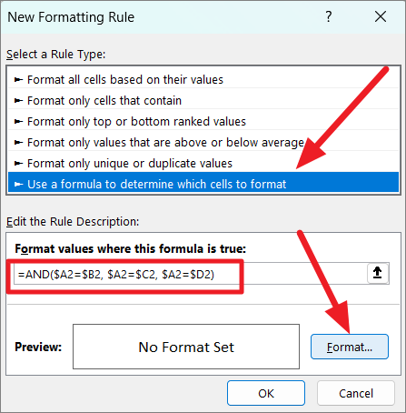
หลังจากนั้น เลือก’ใช้สูตร เพื่อกำหนดประเภทกฎที่จะจัดรูปแบบเซลล์ และป้อนกฎด้านล่างเพื่อไฮไลต์รายการที่ตรงกันในคอลัมน์ A:

=COUNTIF($B$2:$B$12, $A2)>0

จากนั้น คลิกปุ่ม’ปุ่ม Format’เพื่อเลือกการจัดรูปแบบที่คุณต้องการนำไปใช้

คลิก’ตกลง’เพื่อใช้ การจัดรูปแบบเป็นคอลัมน์ A.

ถัดไป เลือกคอลัมน์ B แล้วคลิกตัวเลือก’การจัดรูปแบบตามเงื่อนไข’จากริบบิ้น จากนั้นเลือกตัวเลือก’กฎใหม่’จากเมนู

ในหน้าต่างกฎการจัดรูปแบบใหม่ ให้เลือก’ใช้สูตรเพื่อกำหนดเซลล์ที่จะจัดรูปแบบ’ประเภทของกฎและป้อนด้านล่างเพื่อเน้นรายการที่ซ้ำกันในคอลัมน์ B:

=COUNTIF($A$2:$A$12, $B2)>0

หลังจากป้อน สูตร ให้คลิกปุ่ม’รูปแบบ’และระบุการจัดรูปแบบสำหรับการไฮไลต์เซลล์

หลังจากเลือกรูปแบบแล้ว ให้คลิก’ตกลง’เพื่อนำไปใช้

ตอนนี้ ค่าที่ซ้ำกันในทั้งสองคอลัมน์ได้รับการเน้นแล้ว

เปรียบเทียบสองคอลัมน์และเน้นค่าที่ไม่ซ้ำ

วิธีนี้ตรงกันข้ามกับวิธีการข้างต้น หากคุณต้องการเปรียบเทียบสองคอลัมน์และเน้นเฉพาะค่าที่ไม่ซ้ำในทั้งสองคอลัมน์ที่ไม่ตรงกัน คุณสามารถใช้การจัดรูปแบบตามเงื่อนไขสำหรับสิ่งนี้ได้เช่นกัน

ขั้นแรก เลือกคอลัมน์ที่คุณต้องการเปรียบเทียบ ไปที่’แท็บหน้าแรก แล้วคลิกเมนู’การจัดรูปแบบตามเงื่อนไข’ในกลุ่มสไตล์

จากนั้น วางเมาส์เหนือตัวเลือก’ไฮไลต์กฎของเซลล์’และเลือก’ค่าที่ซ้ำกัน’

ในเมนูดรอปที่ระบุว่าซ้ำ ให้เลือก’ไม่ซ้ำกัน’จากนั้นเลือกการจัดรูปแบบที่กำหนดไว้ล่วงหน้าสำหรับข้อมูลที่ไม่ตรงกัน จากนั้น คลิก’ตกลง’

ตอนนี้ ค่าที่ไม่ซ้ำหรือไม่ตรงกันจากทั้งสองคอลัมน์จะถูกเน้น

p>

อีกวิธีหนึ่ง คุณยังสามารถใช้กฎการจัดรูปแบบที่กำหนดเองเพื่อเน้นค่าที่ไม่ซ้ำในสองคอลัมน์

ในการทำเช่นนั้น ก่อนอื่นให้เลือกคอลัมน์ A แล้วคลิกตัวเลือก’การจัดรูปแบบตามเงื่อนไข’จากริบบิ้น จากนั้นเลือกตัวเลือก’กฎใหม่’จากเมนู

หลังจากนั้น เลือก’ใช้สูตรเพื่อ กำหนดประเภทกฎที่จะจัดรูปแบบเซลล์ และป้อนกฎด้านล่างเพื่อไฮไลต์รายการที่ตรงกันในคอลัมน์ A:

=COUNTIF($B$2:$B$12, $A2)=0

จากนั้น คลิกปุ่ม’รูปแบบ’ปุ่มเพื่อเลือกการจัดรูปแบบ

คลิก’ตกลง’เพื่อใช้การจัดรูปแบบกับคอลัมน์ A

ถัดไป เลือกคอลัมน์ B และคลิกตัวเลือก’การจัดรูปแบบตามเงื่อนไข’จากริบบิ้น จากนั้นเลือกตัวเลือก’กฎใหม่’จากเมนู

ในหน้าต่างกฎการจัดรูปแบบใหม่ ให้เลือก’ใช้สูตรเพื่อกำหนดเซลล์ที่จะจัดรูปแบบ’ประเภทของกฎและป้อนด้านล่างเพื่อเน้นรายการซ้ำในคอลัมน์ B:

=COUNTIF($A$2:$A$12, $B2)=0

หลังจากป้อน สูตร ให้คลิกปุ่ม’รูปแบบ’และระบุการจัดรูปแบบสำหรับการเน้นเซลล์ จากนั้น คลิก’ตกลง’เพื่อนำไปใช้

ตอนนี้ ค่าที่ไม่ซ้ำในทั้งสองคอลัมน์ได้รับการเน้นแล้ว

เปรียบเทียบหลายคอลัมน์และไฮไลต์แถวที่ตรงกัน

เราได้เห็นวิธีเปรียบเทียบสองคอลัมน์และ ไฮไลต์แถวที่ตรงกัน แต่ถ้าคุณมีหลายคอลัมน์ที่ต้องเปรียบเทียบ คุณสามารถทำได้โดยใช้การจัดรูปแบบตามเงื่อนไข ด้วยการจัดรูปแบบตามเงื่อนไข เราสามารถเปรียบเทียบหลายคอลัมน์ ทีละแถว และไฮไลต์รายการที่ตรงกันได้

ตัวอย่างเช่น เรามีรายการผลไม้จากร้านค้าที่แตกต่างกันสามร้าน และเราต้องการเน้นแถวที่มีสินค้าเหมือนกันใน ทั้งสามคอลัมน์ โดยทำตามขั้นตอนต่อไปนี้:

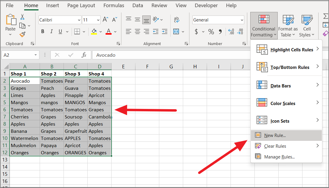
ขั้นแรก ให้เลือกคอลัมน์เพื่อเปรียบเทียบ (A2:D12) Then, click the’Conditional Formatting’menu and select the’New Rule..’option.

To compare multiple ให้สร้างกฎการจัดรูปแบบตามเงื่อนไขใหม่ด้วยฟังก์ชัน AND หรือ COUNTIF:

=AND($A2=$B2, $A2=$C2, $A2=$D2)

ตำแหน่งที่คอลัมน์ A, B และ C ถูกล็อกไว้ในการอ้างอิงแบบสัมบูรณ์โดยใช้เครื่องหมาย $ ในขณะที่หมายเลขแถว (2) ถูกปล่อยให้เป็นข้อมูลอ้างอิงแบบสัมพัทธ์ ดังนั้นสูตรสามารถเปลี่ยนแปลงโดยอัตโนมัติเพื่อเปรียบเทียบค่าทีละแถว เมื่อนำสูตรข้างต้นไปใช้กับตาราง จะเปรียบเทียบแถวแรกของตาราง จากนั้น สูตรจะปรับตัวเองเป็น=AND($A3=$B3, $A3=$C3, $A3=$D3) และอื่นๆ โดยอัตโนมัติ เฉพาะหมายเลขแถวเท่านั้นที่เปลี่ยนแปลงเนื่องจากเป็นการอ้างอิงแบบสัมพัทธ์และตัวอักษรของคอลัมน์ยังคงเหมือนเดิมเนื่องจากเป็นการอ้างอิงแบบสัมบูรณ์

ค่าเซลล์แต่ละค่าในแถวจะถูกเปรียบเทียบกับค่าของคอลัมน์แรก เมื่อตรงตามเงื่อนไขทั้งหมด ฟังก์ชัน AND จะส่งกลับ TRUE หากผลลัพธ์ของกฎการจัดรูปแบบตามเงื่อนไขเป็น TRUE แถวที่เกี่ยวข้องจะถูกเน้นด้วยการจัดรูปแบบที่ระบุ

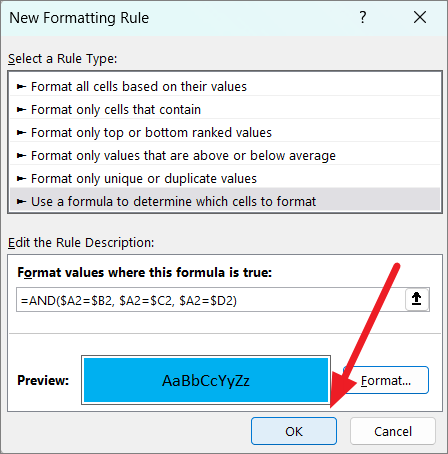
ในหน้าต่างกฎการจัดรูปแบบใหม่ ให้เลือก’ใช้สูตรเพื่อกำหนดเซลล์ที่จะจัดรูปแบบ’และพิมพ์ สูตรข้างต้นในช่องข้อความ’จัดรูปแบบค่าที่สูตรนี้เป็นจริง:’Then, click’Format’to specify formatting.

After selecting the formatting, click’Ok’to apply the conditional formatting.

Now, the rows with the same values ​​in multiple columns are highlighted.

In case you have a lot of columns to compare, you can also use the COUNTIF function to create a conditional formatting rule:

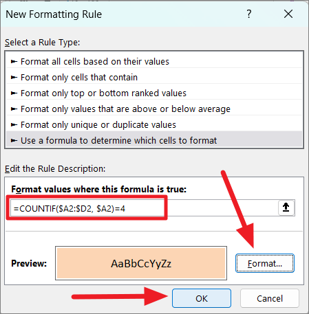
=COUNTIF( $A2:$D2, $A2)=4

จะเปรียบเทียบ A2 อีกครั้ง st ทุกเซลล์ในแถวแรก (A2:D2) และ 4 คือจำนวนคอลัมน์ที่จะเปรียบเทียบ สูตรจะตรวจสอบว่า A2 ตรงกับเซลล์อื่นในแถวหรือไม่ ถ้าแถวมีค่าเหมือนกันในทั้งสี่คอลัมน์ ฟังก์ชัน COUNTIF จะส่งกลับ 4 ถ้าผลลัพธ์ของฟังก์ชัน COUNTIF เท่ากับจำนวนคอลัมน์ (4) กฎการจัดรูปแบบตามเงื่อนไขจะส่งผลให้ TRUE และแถวที่เกี่ยวข้องจะถูกเน้น

กฎการจัดรูปแบบตามเงื่อนไขด้านบนจะปรับตัวเองโดยอัตโนมัติเพื่อเปรียบเทียบแต่ละแถวในตาราง

ในการเริ่มต้น เลือกคอลัมน์สำหรับการเปรียบเทียบ คลิกเมนู’การจัดรูปแบบตามเงื่อนไข’และเลือก’New Rule…’

Next, select the’Use a formula to determine which cells to format’rule type and ป้อนสูตรด้านบนในช่องข้อความด้านล่าง After that, specify the formatting for the highlights and click’OK’.

Now, the rows with the same values in multiple columns are highlighted.

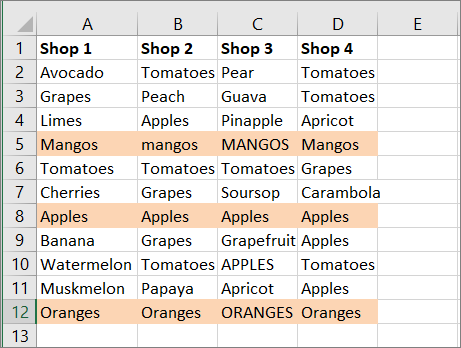
You should know that AND and COUNTIF formulas can be used to compare มากกว่า 4 คอลัมน์และไฮไลต์แถวที่มีค่าเดียวกัน

เปรียบเทียบหลายคอลัมน์และไฮไลต์ความแตกต่างของแถว

หากคุณต้องการเปรียบเทียบหลายคอลัมน์และเน้นค่าที่แตกต่างกัน (ข้อมูลไม่ตรงกัน) ในแต่ละคอลัมน์ คุณสามารถใช้คุณลักษณะ’ไปที่แบบพิเศษ’ใน Excel ได้

ในการดำเนินการนี้ ให้เลือกคอลัมน์ที่คุณต้องการเปรียบเทียบ

In the Go To Special dialog box, select’Row differences’and click the’OK’button.

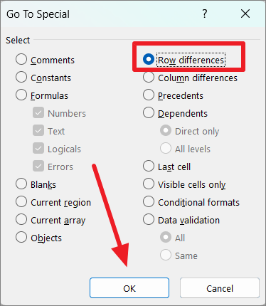
As you can see, all the cell values that are different in the comparison column in each row will be highlighted/selected.

To highlight the selected cells with a color, click the ‘Fill Color’ button on the ribbon and pick a color from the palette.

Compare Two Columns Using VLOOKUP and Extract Matching Data

Sometimes, you may not only want to compare items in one list to the other, but also pull matching data. When comparing columns, there are two types of matches you can use – a partial match or an exact match. This can be done with VLOOKUP or INDEX MATCH function.

The VLOOKUP function is used to search for a specific value in a column and returns a corresponding value from a different column in the same row.

Syntax of VLOOKUP function:

=VLOOKUP(lookup_value,table_array,col_index_num,[range_lookup])

This function consists of 4 parameters or arguments:

lookup_value:  This specifies the value that you are searching for in the first column of the given table array. The Lookup value must always be in the left-most column of the search table. table_array: This is the table (range of cells) in which you want to look up a value. This table (search table) can be in the same worksheet or different worksheet, or even a different workbook. col_index_num: This specifies the column number of the table array that has the value you wish to extract. [range_lookup]: This parameter specifies if you want to extract an exact match or an approximate match. It’s either TRUE or FALSE, enter ‘FALSE’ if you want the exact value or enter ‘TRUE’ if you’re OK with the approximate value.

Exact Match

Let’s assume we have two tables with a list of items. In the second, we have a list of items and their prices need to be filled. To do that, we need to compare column A with column D and extract prices for the matching items.

We can use the VLOOKUP function to compare two columns and fetch matching data:

=VLOOKUP(D2,$A$2:$B$13,2,FALSE)

First, enter the formula in cell E2 and then copy the formula down the column by dragging the fill handle.

Where D2 is the value that needs to be searched in the first column of the lookup table. $A$2:$B$13 represents the lookup table where the value will be searched and the corresponding value will be pulled. Here the range is locked into absolute references to prevent the cell reference from changing as the formula is copied down.

The ‘2’ in the formula is the column number of the lookup table with the value you wish to extract. The FALSE parameter is used to find the exact match of D2.

The above formula will search the first column of the range A2:B13 (column A) for the value in D2. An exact match of D2 is found in row 5 of column A, so the corresponding value is extracted from column B (column 2) and returned in E2. When the formula is copied down column E, only the lookup_value value automatically adjusts to D3, D4, etc to search each value of column D in the range A2:B13.

Compare Columns and Pull Matching Data using IFERROR or IFNA functions

In case the lookup_value is not found in the lookup table or the look_up value weren’t exact copies of the values in the look_up table, you would get the #N/A error.

In the below example, lookup_values (D3 and D5) weren’t found in column A and the match type is FALSE (exact), so the formula returns the #N/A error.

This can happen even if there is an extra space, missing space, or a typo in the look_up value. In such cases, you can change the match_type to TRUE which will enable the formula to ignore small errors and look for an approximate match of the values.

If the lookup_value is not found in the table, you can use IFNA or IFERROR function to avoid the #N/A error.

=IFNA(VLOOKUP(D2,$A$2:$B$13,2,FALSE),””)

This formula works the same way as the previous VLOOKUP formula, except the IFNA replaces the error message with a blank. You can also have the formula return a text instead of a blank cell.

Alternatively, you can also use the IFERROR function to remove the error message and return a specified text string. To do that, enter the below formula:

=IFERROR(VLOOKUP(D2,$A$2:$B$13,2,FALSE),”Not Available”)

Enter the above formula in cell E2 and copy it down the column. If the VLOOKUP function returns an #N/A error, then the IFERROR function replaces it with the “Not Available” message as shown below.

Compare Two Columns and Find a Partial Match using Wildcards

In case there are minor differences in the names in the two columns, the TRUE parameter in the VLOOKUP function won’t cover it. For example, if one column has a value called “Google” and the other has “Google LLC”, the above VLOOKUP formula won’t be able to match the columns. However, you can still use the VLOOKUP to partially match columns by adding wildcards to the formula.

The VLOOKUP function allows you to find a partial match on a specified value using wildcard characters. If you want to locate a value that contains the lookup value in any position, add an ampersand sign (&) to join the lookup value with the wildcard character (*). Use ‘$’ signs to make absolute cell references and add the wildcard ‘*’ sign before or after the lookup value.

In the below example, we only have part of a lookup value (Fan) in cell D3. So, to perform a partial match on the given characters, concatenate a wildcard ‘*’ before and after the cell reference.

=VLOOKUP(“*”&D3&”*”,$A$2:$B$13,2,FALSE)

In the above formula, D2 has been enclosed in ‘&’ operators and asterisks “*” to make up for the missing character before and after the lookup value. If List 2 doesn’t have the entire name of the items, the asterisks characters will make up for the missing characters and pull values from the partially matched columns.

For instance, in cell D3 we only have the item named ‘Fan’ but in column A we have ‘Table Fan’. But the asterisks ‘*’ before the D3 made up for the missing ‘Table’ before the lookup value. So, the VLOOKUP function returns the corresponding value ‘31.68’ from column B.

Compare Two Columns using the MATCH Function

If you want to return the position of the matching value in the column instead of the value itself, you can use the MATCH function.

The MATCH function is a built-in function in Excel and its primarily used for locating the relative position of a lookup value in a column or a row.

Syntax of MATCH Function:

=MATCH(lookup_value,lookup_array,[match_type})

Where:

lookup_value – The value you want to look up in a specified range of cells or an array. It can be a numeric value, text value, logical value, or a cell reference that has a value.

lookup_array – The arrays of cells in which you are searching for a value. It must be a single column or a single row.

match_type – It is an optional parameter that can be set to 0,1, or-1 and the default is 1.

0 looks for an exact match, and when it’s not found, returns an error. -1 looks for the smallest value that is greater than or equal to lookup_value when the lookup array is in ascending order. 1 looks for the largest value that is less than or equal to the look_up value when the lookup array is in descending order.

Compare Two Columns and Find the Position of An Exact Match

Let’s assume, we have the following tables where we want to find the position of each value in column D in column A.

=MATCH(D2,$A$2:$A$13,0)

The formula searches for each value of list 2 in list 1 and returns the position of each value.

Display Duplicates or Matching Data using the MATCH function

A combination of MATCH, ISERROR, and IF functions can be used to compare and display duplicates of columns.

For example, we can use the below formula to compare the two columns and display duplicates in the first column:

=IF(ISERROR(MATCH(A2,$B$2:$B$10,0)),””,A2)

Here, the ISERROR function is combined with the IF function to find errors and display text strings or blanks.

The MATCH function searches and returns the position of A2 (in the range B2:B10) as 5. Since it is not an error, the ISERROR function returns FALSE, and the IF function returns the value of A2. In another instance, the MATCH function in C6 returns a #N/A error because the value of A6 is not found in the range B2:B10. Hence, the ISERROR function returns TRUE, and subsequently, the IF function returns the blank.

Display Unique Data using the MATCH function

If you want to compare two columns and display the unique values in each column, you can also do that with the same above formula by simply swapping the last 2 arguments of the IF function.

To display unique values in the first column, enter the below formula:

=IF(ISERROR(MATCH(A2,$B$2:$B$10,0)),A2,””)

The MATCH function searches and returns the position of A2 (in the range B2:B10) as 5. Since the result is not an error, the ISERROR function returns FALSE and the IF function returns the blank space.

The MATCH function in C4 returns a #N/A error because the value of A4 is not found in the range B2:B10. Hence, the ISERROR function returns TRUE, and subsequently, the IF function returns the value of A4.

To display unique values in the second column, enter the below formula:

=IF(ISERROR(MATCH(B2,$A$2:$A$10,0)),B2,””)

The MATCH function looks at and returns the position of B2 (in the range A2:A10) as 5. Since the result is not an error, the ISERROR function returns FALSE and the IF function returns the blank space.

The MATCH function in C4 returns a #N/A error because the value of B4 is not found in the range B2:B10. Hence, the ISERROR function returns TRUE, and subsequently, the IF function returns the value of B4.

Compare Two Columns using INDEX and MATCH Functions

The MATCH function can be combined with the INDEX function to compare and match two columns. Compared to VLOOKUP, the INDEX MATCH is a powerful and versatile formula that can compare two columns and also pull the matching data.

The INDEX function is used to retrieve a value at a specific location in a table or a range. The MATCH function returns the relative position of a value in a column or a row. When combined, the MATCH finds the row or column number (location) of a specific value, and the INDEX function retrieves a value based on that row and column number.

Syntax of INDEX function:

=INDEX(array,row_num,[col_num],) array – The arrays of cells in which you are searching for a value. row_num –  It represents the row in the array from which to return a value. If row_num is omitted, column_num is required. column_num – It represents the column in the array from which to return a value. If column_num is omitted, row_num is required.

Example:

To compare the two columns A and D and fetch the price (the matched value) for column D by using INDEX and MATCH:

=INDEX($B$2:$B$13,MATCH(D2,$A$2:$A$13,0))

Enter the formula in cell E2 and copy it down the range E3:E7. Now, let’s see how the formula works:

INDEX function needs a row and column number to retrieve a value. In the above formula, the nested MATCH function finds the row number (position) of the value D2. Then we supply that row number (5) to the INDEX function with a range B2:B13. We specified ‘0’ as the last argument to ignore the column number because we are considering only one column in our array, column B ($B$2:$B$13).

Finally, the INDEX function returns the 5th value in the array B2:B13, which is 24.14.

As you can see, we encountered the #N/A errors in cell E5 because the cell value D5 is not available in column A. To avoid such errors, you can wrap the formula with an IFERROR function.

=IFERROR(INDEX($B$2:$B$13,MATCH(D2,$A$2:$A$13,0)),””)

Using Wildcards

In case there is little difference in the names in the two columns that we are comparing, you can partially match columns by adding wildcards to the formula.

Wildcards can be used in the MATCH function only when match_type is set to ‘0’ and the lookup value is a text string. There are wildcards you can use in the MATCH function: an asterisk (*) and a question mark (?).

Question mark (?) is used to match any single character or letter with the text string. Asterisk (*) is used to match any number of characters with the string.

As you can see below, the names in List 2 are not as complete as in List 1, so using wildcards can make up for the missing characters.

=INDEX($B$2:$B$13,MATCH(“*”&D2&”*”,$A$2:$A$13,0))

In the above formula, D2 has been enclosed in ‘&’ operators and asterisks “*” to make up for the missing character before and after the lookup value. If list 2 doesn’t have the entire name of the items, the asterisks characters will make up for the missing characters and extract values from the partially matched columns.

Compare Two Columns and Find Matches and Differences using VBA Macro

In case you need to compare and match columns often or repeatedly, you can create VBA Macros to automate those tasks. You can use VBA code to create custom user-generated functions to perform tasks and calculations. Here’s how you can do that:

Compare Two Columns Row by Row and Highlight Differences using VBA Code

VBA Macro is the quickest and most effective way to compare two columns in Excel. If you want to compare two columns and highlight the differences between them, follow the instructions:

First, open the workbook that contains the two columns you want to compare.

Then, go to the ‘Developer’ tab and click the ‘Visual Basic’ option from the ribbon or press Alt+F11 keyboard shortcut to open Microsoft Visual Basic for Applications.

This will open Microsoft Visual Basic for Applications in a separate window. In the VBA window, click the ‘Insert’ menu and select the ‘Module’ option. Alternatively, you can just right-click on the ‘Microsoft Excel Objects’ in the navigation bar on the left, click ‘Insert’, and then select ‘Module’ from the sub-menu.

Now, copy and paste the following VBA script into the new module window:

Sub HighlightColumnDifferences() Dim Rg As Range Dim Ws As Worksheet Dim FI As Integer On Error Resume Next SRC: Set Rg=Application.InputBox(“Select Two Columns:”,”Excel”, , , , , , 8) If Rg Is Nothing Then Exit Sub If Rg.Columns.Count <> 2 Then MsgBox”Please Select Two Columns” GoTo SRC End If Set Ws=Rg.Worksheet For FI=1 To Rg.Rows.Count If Not StrComp(Rg.Cells(FI, 1), Rg.Cells(FI, 2), vbBinaryCompare)=0 Then Ws.Range(Rg.Cells(FI, 1), Rg.Cells(FI, 2)).Interior.ColorIndex=6’you can change the color index as you like. End If Next FI End Sub

The above code allows you to compare two columns row by row and highlight the differences between them.

After pasting the script, click ‘File’ and select ‘Save XXXX (filename)’ to save this module as a macro.

The VB script needs to be saved in a macro-enabled file type. Once you click ‘Save’, you will see a prompt box asking whether you want to save this file in a macro-free file or macro-enabled file type.

Click ‘No’ to choose the macro-enabled file type.

In the Save As window, choose the ‘Excel Macro-Enabled Workbook (*.xlsm)’ format from the ‘Save As type’ drop-down.

Then, click the ‘Save’ button to save the VBA macro with the workbook.

Now, you can run the macro to compare columns.

Go back to your Excel worksheet, then he ad to the ‘Developer’ tab in ‘Ribbon’ and select ‘Macros’ or press ALT+F8.

A dialog box named Macro will open up. Under the Macro name, you will see the macro you created. Select the ‘HighlightColumnDifference’ macro and click ‘Run’.

Now, you will see a dialog box for specifying the two columns. Simply select the columns you want to compare and click ‘OK’.

The differences between the two columns will be highlighted with a background color you specified in the code. This VBA code compares columns with case-sensitive and highlights the differences.

Compare Two Columns and Highlight Matching Data (or Duplicates) using VBA Code

If you want to compare two columns and then highlight the matches or duplicates in the second column, you can use the below code.

Open the spreadsheet and press Alt+F11 to open the Microsoft Visual Basic for Applications window. Then, go to ‘Insert’ > ‘Module’ in the Microsoft Visual Basic for Applications window.

Next, copy-paste the below macro code into the new blank Module script:

Sub CompareTwoRanges() Dim xRg, xRgC1, xRgC2, xRgF1, xRgF2 As Range SRg: Set xRgC1=Application.InputBox(“Select the column you want compare according to”,”Excel”, , , , , , 8) If xRgC1 Is Nothing Then Exit Sub If xRgC1.Columns.Count <> 1 Then MsgBox”Please select a single column” GoTo SRg End If SsRg: Set xRgC2=Application.InputBox(“Select the column you want to highlight duplicates in:”,”Excel”, , , , , , 8) If xRgC2 Is Nothing Then Exit Sub If xRgC2.Columns.Count <> 1 Then MsgBox”Please select a single column” GoTo SsRg End If For Each xRgF1 In xRgC1 For Each xRgF2 In xRgC2 If xRgF1.V alue=xRgF2.Value Then xRgF2.Interior.ColorIndex=38′(you can change the color index as you need) End If Next Next End Sub

After pasting the code save the file as a Macro-Enabled Workbook with ‘*.xlsm’ format like we showed you above. Then, close the module and Microsoft Visual Basic for Applications window.

To run the VBA macro, switch to the ‘Developer’ tab and click ‘Macros’ from the Code group.

In the Macro dialog window, select ‘CompareTwoRanges’ and click ‘Run’.

When you see the first pop-up dialog box, select the column that you want to compare duplicate values according to and click ‘OK’.

In the second dialog box, select the column where you want to highlight duplicate values and click ‘OK ’.

As you can see below, the second column is compared against the first column, and duplicates are highlighted in the second column with a background color. This VBA code compares columns with case-sensitive matches.

Compare Two Columns and Extract Matching Data using VBA Code

In case you want to compare two columns row by row and pull the matching values (duplicates) to another column, you can use the below macro code.

Open a blank module in the Microsoft Visual Basic for Applications window as we showed you. Copy and paste the below script to the new blank module:

Sub PullMatches() Dim xRg, xRgC1, xRgC2, xRgF1, xRgF2 As Range Dim xIntSR, xIntER, xIntSC, xIntEC As Integer On Error Resume Next SRg: Set xRgC1=Application.InputBox(“Select first column:”,”Excel”, , , , , , 8) If xRgC1 Is Nothing Then Exit Sub If xRgC1.Columns.Count <> 1 Then MsgBox”Please select single column” GoTo SRg End If SsRg: Set xRgC2=Application.InputBox(“Select the second column:”,”Excel”, , , , , , 8) If xRgC2 Is Nothing Then Exit Sub If xRgC2.Columns.Count <> 1 Then MsgBox”Please select single column” GoTo SsRg End If Set xWs=xRg.Worksheet For FI=1 To xRg.Rows.Count If Not StrComp(xRg.Cells(FI, 1), xRg.Cells(FI, 2), vbBinaryCompare)=0 Then Ws.Range(xRg.Cells(FI, 1), Rg.Cells(FI, 2)).Interior.ColorIndex=8’you can change the color index as you like. End If Next FI End Sub

After pasting the code save the file and close the Microsoft Visual Basic for Applications window. Then, open the Marco dialog window, select the ‘PullMatches’ macro and click ‘Run’.

First, select the first column (left) you want to compare and click ‘OK’.

In the second dialog, select the second column you want to compare and click ‘OK’.

The matches between two columns will be pulled and displayed automatically in the right column of the two columns you selected.

Compare Two Columns and Extract Unique Data using VBA Code

If you want to two compare columns and pull unique values, here’s the below VBA code that can help you.

Open a blank module in the Microsoft Visual Basic for Applications window and copy-paste the below script to the new blank module:

Sub PullUniques() Dim xRg, xRgC1, xRgC2, xFRg1, xFRg2 As Range Dim xIntR, xIntSR, xIntER, xIntSC, xIntEC As Integer Dim xWs As Worksheet On Error Resume Next SRg: Set xRg=Application.InputBox(“Select two columns:”,”Excel”, , , , , , 8) If xRg Is Nothing Then Exit Sub If xRg.Columns.Count <> 2 Then MsgBox”Please select two columns as a range” GoTo SRg End If Set xWs=xRg.Worksheet xIntSC=xRg.Column xIntEC=xRg.Columns.Count + xIntSC-1 xIntSR=xRg.Row xIntER=xRg.Rows.Count + xIntSR-1 Set xRg=xRg.Columns Set xRgC1=xWs.Range(xWs.Cells(xIntSR, xIntSC), xWs.Cells(xIntER, xIntSC)) Set xRgC2=xWs.Range(xWs.Cells(xIntSR, xIntEC), xWs.Cells(xIntER, xIntEC)) xIntR=1 For Each xFRg In xRgC1 If WorksheetFunction.CountIf(xRgC2, xFRg.Value)=0 Then xWs.Cells(xIntER, xIntEC).Offset(xIntR)=xFRg xIntR=xIntR + 1 End If Next xIntR=1 For Each xFRg In xRgC2 If WorksheetFunction.CountIf(xRgC1, xFRg)=0 Then xWs.Cells(xIntER, xIntSC).Offset(xIntR)=xFRg xIntR=xIntR + 1 End If Next End Sub

Then save the file and close the Microsoft Visual Basic for Applications window.

After that, open the Marco dialog window, select the ‘PullUniques’ macro, and click ‘Run’.

In the pop-up window, select the two comparing columns and click ‘OK’.

The Macro compares columns without case sensitivity and lists unique values from the two columns.

That’s it. Now, you know everything about comparing columns in Excel. You can opt for the method that suits you the best.