O guia completo para comparar duas colunas no Excel e obter correspondências ou diferenças, realçá-las ou até mesmo extrair os dados.
Quando você está trabalhando com dados no Excel , talvez seja necessário comparar colunas para encontrar semelhanças e diferenças entre os dados. Comparar colunas é muito útil para organizar e analisar dados. Comparar manualmente os dados de duas colunas pode ser uma tarefa demorada e exaustiva, então você pode usar várias fórmulas do Excel para corresponder colunas.
O Excel tem vários métodos e funções para comparar colunas e encontrar dados correspondentes e incompatíveis. Você pode usar operadores lógicos – VLOOKUP, MATCH, AND, INDEX, IF, COUNTIF, ISERROR, SEERRO – ou regras de formatação condicional para comparar e corresponder dados. Neste artigo, discutiremos diferentes métodos para comparar colunas no Excel para correspondências e diferenças.
Comparação de duas colunas linha por linha para correspondências ou diferenças
A maneira mais simples de comparar duas colunas no Excel é uma simples comparação linha por linha, linha por linha. Este método verifica se o valor em uma coluna corresponde ao valor em outra coluna na mesma linha. Ele só comparará valores na mesma linha, não todo o conjunto de dados. Existem diferentes tipos de fórmulas que você pode usar para comparar duas colunas linha por linha-usando um operador de comparação simples, uma função SE e uma função EXATA.
Comparar colunas usando o operador Equals
O A maneira mais fácil de comparar os dados de duas colunas linha por linha para encontrar a correspondência é usando o operador de comparação. Com o’Igual a'(=), você pode comparar células em duas colunas para uma correspondência e obter o resultado como verdadeiro ou falso.
Exemplo 1:
Por exemplo, compararemos duas colunas (Fatura vencida e Conta paga na captura de tela abaixo) para ver se elas correspondem. Para fazer isso, usaremos a fórmula simples abaixo:
=B2=C2
O valor em B2 corresponde ao valor em C2, então a fórmula retorna TRUE. Primeiro, insira a fórmula na célula D2 e copie-a para outras células arrastando a alça de preenchimento para comparar as colunas B e C linha por linha. A alça de preenchimento é um pequeno quadrado verde no canto inferior direito da célula selecionada.
Quando você arrasta o preencha a alça da célula D2 a D12, o cursor se transformará em um sinal de mais preto.
Ao aplicar o fórmula através das células D2 a D12, ele comparará os valores linha por linha e você verá algumas correspondências de linhas enquanto outras não. Por exemplo, o valor da célula B4 não corresponde à célula adjacente C4, portanto, o valor na célula D4 é FALSE.
Exemplo 2:
Vimos como a fórmula acima lida com números, mas também pode comparar datas, horas e strings de texto igualmente bem. Vamos ver como a fórmula compara colunas com valores de texto.
=A2=B2
A fórmula procura a correspondência correta entre as duas colunas e não perderá nem um único caractere de espaço. Em seguida, ele retorna TRUE se a condição for atendida ou então retorna FALSE. O endereço de cobrança na célula A2 corresponde ao endereço de entrega na célula B2, como resultado, obtemos TRUE. Além disso, o endereço na célula A5 não corresponde ao endereço na célula B5 – o último caractere é diferente na célula B5. Portanto, ele retorna FALSE.
Comparar colunas usando a função IF
Outra maneira de podermos comparar duas colunas linha por linha é usando a função SE. A função SE verifica se uma condição ou critério é atendido e retorna um valor especificado se a condição for TRUE ou outro valor se a condição for FALSE. Embora esse método seja semelhante ao método acima, podemos usá-lo para obter resultados mais descritivos do que apenas VERDADEIRO ou FALSO.
Por exemplo, podemos usar a fórmula abaixo para comparar duas colunas e, se houver um correspondência, podemos obter o resultado”Pago”ou”Não pago”se não houver correspondência:
=IF(B2=C2,”Pago”,”Não pago”)
Na fórmula acima, o A função SE verifica se o valor em B2 é igual ao valor em C2, e se a condição for True, retorna o texto “Pago”. Se a condição for False, retorna “Not Paid”. O valor da fatura em B2 e o valor da fatura em C2 são os mesmos, então ele retorna “Pago” em D2. Mas o valor em B5 e C5 não corresponde, então a fórmula retorna”Não pago”em D5.
Somente para correspondências:
Caso você queira encontrar apenas correspondências em duas colunas, use a fórmula abaixo:
=IF(B2=C2,”Pago”,””)
A fórmula acima verifica se o valor na coluna B é igual aos valores na coluna C, linha por linha. Se a condição for verdadeira, obteremos a string de texto “Pago” e se a condição for falsa, não obteremos nada (string vazia).
Somente para diferenças:
Para localizar células com valores diferentes na mesma linha, tente a fórmula abaixo:
=IF( B4<>C4,”Não Pago”,””)
A fórmula acima verifica se os valores da coluna B não são iguais aos valores da coluna C, linha por linha. Se a condição for verdadeira, obteremos a string de texto “Não pago” e se a condição for falsa, não obteremos nada (string vazia).
Observação: as fórmulas de igual a fórmula e função SE não diferenciam maiúsculas de minúsculas, o que significa que elas ignorarão maiúsculas e minúsculas ao comparar valores de texto.
Compare Duas colunas para correspondência sensível a maiúsculas e minúsculas na mesma linha usando a função EXACT
As fórmulas acima ignoram casos ao comparar valores de texto. Se você quiser fazer a comparação com distinção entre maiúsculas e minúsculas, você precisa usar a função EXACT. A função EXACTA do Excel é usada para comparar duas strings de texto e retorna TRUE se ambos os valores forem iguais e FALSE caso contrário. Você pode usar EXACT sozinho ou com a função SE (caso queira obter um resultado descritivo em vez de apenas VERDADEIRO ou FALSO.
Por exemplo, vamos comparar listas de nomes de empresas de diferentes bancos de dados e ver se eles são correspondências exatas usando a função EXACT simples:
=EXACT(A2,B2)
A fórmula acima verifica se as strings de texto de A2 e B2 são uma correspondência exata que diferencia maiúsculas de minúsculas. Em seguida, ela retorna FALSE porque a palavra “St” em A2 está em letras minúsculas enquanto em B2, em maiúscula.
Caso queira para obter resultados descritivos, você precisa usar a função SE com a função EXACT:
=IF(EXACT(A3,B3),”Match”,”Check Database”)
Na fórmula acima, o EXACT A função verifica se os valores nas células A3 e B3 são correspondências exatas com distinção entre maiúsculas e minúsculas. No entanto, a primeira palavra’ANGELO’é maiúscula em B2 que é diferente do nome da empresa em A2, então a função EXACT retorna FALSE. Portanto, a função IF retorna a string de texto “Check Database” para a saída FALSE.
Na linha 5, os valores de célula A5 e B5 diferenciam maiúsculas de minúsculas, portanto, a função SE obtém um resultado VERDADEIRO da função EXATA e retorna”CORRESP”em seu lugar.
Compare duas colunas se maior que ou menor que
h2>
Às vezes, você pode querer comparar colunas e verificar se os valores em uma coluna são maiores ou menores do que as outras colunas. Por exemplo, se você tiver duas colunas de datas e quiser comparar qual data é posterior na mesma linha (talvez para comparar a data de validade dos produtos), você pode usar uma operação lógica simples para descobrir.
Para saber se os produtos estão vencidos ou não, compare duas colunas se a coluna C for maior que a coluna B:
=IF(C2>B2,”Sim”,”Não”)
A fórmula acima verifica se o valor na célula C2 é maior que a célula B2. Se for TRUE, a função IF retornará’Sim’, caso contrário,’Não’.
Comparar várias colunas Linha por linha para correspondências
Vimos como comparar duas colunas linha por linha, mas você também pode comparar várias colunas para correspondências na mesma linha. Há duas maneiras de comparar várias colunas: encontre correspondências em todas as células na mesma linha ou encontre correspondências em quaisquer duas células na mesma linha.
Encontre correspondências em todas as células na mesma linha
Método 1: se você tiver um conjunto de dados com mais de duas colunas (várias colunas) e quiser encontrar linhas com os mesmos valores em todas as colunas. Você pode fazer isso com as funções IF e AND:
=IF(AND(A3=B3,A3=C3),”All Match”,””)
A função AND testa várias condições ao mesmo (A3=B3 e A3=C3) e retorna TRUE somente se todos os seus argumentos forem avaliados como TRUE. A função AND retornará FALSE mesmo se um dos argumentos for avaliado como FALSE. Você pode adicionar várias condições na função AND incluindo uma vírgula entre cada condição.
Como você pode ver abaixo, a função AND retornará true se todas as células tiverem o mesmo valor na mesma linha. Em seguida, a função IF retornará o texto “All Match” se a função AND retornar TRUE.
Método 2: se seu conjunto de dados tiver muitas colunas, você pode usar a função CONT.SE para tornar sua fórmula compacta:
=IF(CONT.SE($A3:$D3, $A3)=4,”All match”,””)
Onde 4 representa o número de colunas que você está comparando na fórmula. A função CONT.SE é usada para contar os números que atendem a um único critério específico.
A fórmula CONT.SE verifica se a linha tem os mesmos valores em todas as células (A3:D3) e retorna o número total de correspondências. E se todas as colunas corresponderem na mesma linha (o resultado da função CONT.SE) for igual ao número de colunas, você obterá a string de texto que diz “All match”.
Encontre correspondências em quaisquer duas células na mesma linha
Método 1: Suponha que você tenha vários (3 ) e você deseja encontrar correspondências em qualquer uma das duas colunas na mesma linha, você pode fazer isso com a ajuda das funções IF e OR. Para fazer isso, podemos usar a fórmula abaixo:
=IF(OR(A3=B3, B3=C3, A3=C3),”Match”,””)
Na fórmula acima, a função OR compara cada coluna com outras colunas e, se qualquer uma das duas ou mais colunas com o mesmo valor corresponder na mesma linha, retornará TRUE. A função IF retornará o texto’Match’quando for TRUE da função OR.
Método 2: Se você tiver muitas colunas para comparar, a fórmula OR acima pode ficar muito grande e complicada. Para evitar isso, você pode adicionar várias funções CONT.SE:
=SE(CONT.SE(B3:D3,A3)+CONT.SE(C3:D3,B3)+(C3=D3)=0,”Único”,”Match”)
Aqui, a primeira função COUNTIF verifica e conta quantas células (colunas) têm o mesmo valor que a primeira coluna (A3), e a segunda função COUNTIF verifica quantas colunas têm os mesmos valores que a segunda coluna , e assim por diante. Em seguida, todos os resultados da função CONT.SE são somados. Portanto, se a contagem final for igual a 0, a fórmula retornará a string de texto ‘Única’. Se a contagem for diferente de 0, obteremos’Match’como resultado.
Comparar e destacar Colunas correspondentes/incompatíveis
Se você deseja comparar duas colunas e destacar as linhas que têm dados correspondentes ou dados incompatíveis em vez de mostrar o resultado em uma coluna separada, você pode usar a formatação condicional no Excel. A formatação condicional é um recurso do Excel que pode destacar dados com base em um conjunto de regras. Com a formatação condicional, você pode identificar visualmente valores correspondentes ou valores diferentes em duas colunas.
Compare duas colunas e destaque dados correspondentes na mesma linha (lado a lado)
Se desejar para comparar duas colunas e destacar os dados idênticos nas mesmas linhas, siga as etapas abaixo:
Primeiro, selecione as células que deseja comparar e realce. Você pode escolher uma única coluna ou várias colunas se quiser destacar linhas inteiras.
Em’Home’, clique no menu’Formatação condicional’no grupo Estilos e selecione a opção’Nova regra…’no menu.
Isso abrirá a caixa de diálogo Nova regra de formatação. Nessa janela de diálogo, selecione o tipo de regra’Usar uma fórmula para determinar quais células formatar’.
Depois que, digite a seguinte fórmula no campo’Formatar valores onde esta fórmula é verdadeira:’:
=$A1=$B1
Como você pode ver, esta é uma fórmula simples’igual a’que verifica se o valor na célula A1 é igual a B1. Mas adicionamos o sinal’$’antes dos rótulos de coluna A e B para bloquear as colunas em referências absolutas. Portanto, apenas o número da linha muda automaticamente para cada linha quando a fórmula é aplicada.
A seguir, clique no botão Botão”Formatar”para personalizar a aparência desejada para as linhas destacadas.
Na janela de diálogo Formatar células, você pode alterar o tamanho da fonte, a cor da fonte, as bordas da célula, o formato do número etc. Para destacar a correspondência linhas com cores de fundo diferentes, mude para a guia Preenchimento e escolha a cor na seção Cor de fundo. Você também pode alterar o estilo do padrão e a cor do padrão das células realçadas. Quando terminar de escolher o formato, clique no botão’OK’.
Novamente, clique em’OK’em a caixa de diálogo Nova Regra de Formatação para aplicar a formatação
As células com valores correspondentes nas colunas A e B serão ser destacado conforme mostrado abaixo.
Se houver menos dados correspondentes do que dados incompatíveis na tabela, você pode inverter a condição para destacar a diferença de dados entre as duas colunas.
Por exemplo, podemos usar qualquer uma das regras de formatação condicional abaixo para destacar a diferença entre as colunas A e B:
=$A1<>$B1
ou
=$A1=$B1=FALSE
Primeiro, selecione o conjunto de dados e abra a janela Nova regra de formatação, como mostramos acima, e selecione o tipo de regra’Usar uma fórmula para determinar quais células formatar’. Em seguida, insira uma das regras acima e clique no botão’Formatar’.
Em seguida, escolha a formatação desejada deseja aplicar e clique em’OK’. E clique em’OK’novamente para aplicar a formatação.
Comparar duas colunas e destacar valores duplicados
Se você quiser comparar duas colunas e destacar os valores existentes em ambas as colunas mesmo quando não estiverem na mesma linha, use as regras de formatação condicional predefinidas ou regras de formatação personalizadas.
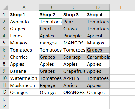
Para Por exemplo, temos duas listas de frutas de diferentes lojas e queremos destacar as frutas que estão disponíveis em ambas as lojas. Veja como fazer isso:
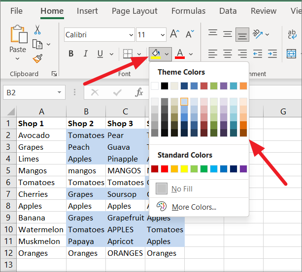
Primeiro, selecione as colunas que deseja comparar e clique no menu”Formatação condicional”no grupo Estilos.
Em seguida, passe o cursor sobre a opção’Destacar Regras de Célula’no menu suspenso e selecione a opção Opção’Valores duplicados’.
Na caixa de diálogo Duplicar Valores, selecione’Duplicar’no lado esquerdo-down.
Em seguida, selecione o formato no menu suspenso do lado direito e clique em’OK’.
Os itens que t existir em ambas as colunas será realçado.
Como alternativa, você também pode usar regras de formatação personalizadas para destacar valores duplicados em duas colunas.
Para fazer isso, primeiro, selecione a coluna A e clique na opção’Formatação Condicional’na faixa de opções. Em seguida, selecione a opção’Nova regra’no menu.
Depois disso, selecione a opção’Usar uma fórmula para determinar quais células devem ser formatadas, digite a regra abaixo para destacar as correspondências na coluna A:
=COUNTIF($B$2:$B$12, $A2)>0
Em seguida, clique no botão’Formato’para selecionar a formatação que deseja aplicar e aplicá-la.
Clique em’Ok’para aplicar o formatação para a coluna A.
Em seguida, selecione a coluna B e clique na opção’Formatação Condicional’na faixa de opções. Em seguida, selecione a opção’Nova regra’no menu.
Na janela Nova regra de formatação, escolha a opção Tipo de regra’Usar uma fórmula para determinar quais células formatar’e digite o seguinte para destacar duplicatas na coluna B:
=CONT.SE($A$2:$A$12, $B2)>0
Depois de inserir o fórmula, clique no botão’Formatar’e especifique a formatação para destacar as células.
Após escolher o formato, clique’OK’para aplicá-lo.
Agora, os valores duplicados em ambas as colunas foram destacados.
Compare duas colunas e realce valores únicos
Este método é exatamente o oposto do método acima. Se você quiser comparar duas colunas e destacar apenas valores únicos em ambas as colunas que não correspondem, você também pode usar a formatação condicional para isso.
Primeiro, selecione as colunas que deseja comparar, vá para”Página inicial”e clique no menu”Formatação condicional”no grupo Estilos .
Em seguida, passe o mouse sobre as opções de’Destacar regras de célula’ e selecione’Duplicar valores’.
No menu suspenso que diz Duplicar, selecione ‘Único’e escolha a formatação predefinida para os dados incompatíveis. Em seguida, clique em’OK’.
Agora, os valores exclusivos ou incompatíveis de ambas as colunas são destacados.
p>
Como alternativa, você também pode usar regras de formatação personalizadas para destacar valores exclusivos em duas colunas.
Para fazer isso, primeiro, selecione a coluna A e clique na opção’Formatação Condicional’na faixa de opções. Em seguida, selecione a opção’Nova regra’no menu.
Depois disso, selecione’Usar uma fórmula para determine quais células devem ser formatadas’tipo de regra e insira a regra abaixo para destacar as correspondências na coluna A:
=CONT.SE($B$2:$B$12, $A2)=0
Em seguida, clique no botão’Formatar’para escolher a formatação.
Clique em’Ok’para aplicar a formatação à coluna A.
Em seguida, selecione a coluna B e clique na opção’Formatação condicional’na faixa de opções. Em seguida, selecione a opção’Nova regra’no menu.
Na janela Nova regra de formatação, escolha a opção Tipo de regra’Usar uma fórmula para determinar quais células formatar’e digite o seguinte para destacar duplicatas na coluna B:
=CONT.SE($A$2:$A$12, $B2)=0
Depois de inserir o fórmula, clique no botão’Formatar’e especifique a formatação para destacar as células. Em seguida, clique em’OK’para aplicá-lo.
Agora, os valores exclusivos em ambas as colunas foram destacados.
Comparar várias colunas e destacar linhas correspondentes
Vimos como comparar duas colunas e realce correspondências de linha, mas se você tiver várias colunas que precisam ser comparadas, também poderá fazer isso com a ajuda da formatação condicional. Com a formatação condicional, podemos comparar várias colunas, linha por linha, e destacar as correspondências.
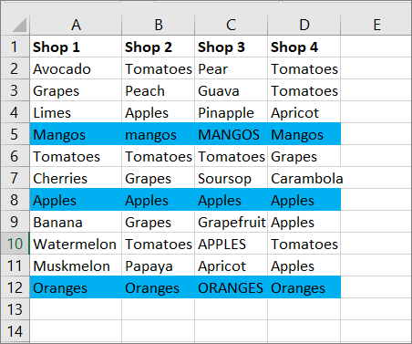
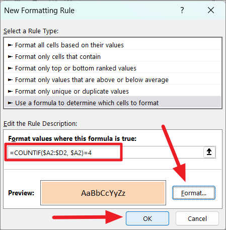
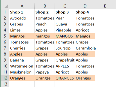
Por exemplo, temos listas de frutas de três lojas diferentes e queremos destacar as linhas que possuem itens idênticos em todas as três colunas. Para fazer isso, siga estas etapas:
Primeiro, selecione as colunas para comparação (A2:D12). Then, click the’Conditional Formatting’menu and select the’New Rule..’option.
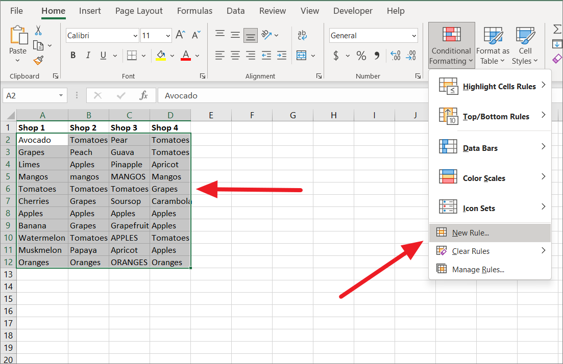
To compare multiple colunas, crie uma nova regra de formatação condicional com a função AND ou COUNTIF:
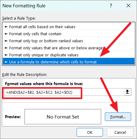
=AND($A2=$B2, $A2=$C2, $A2=$D2)
Onde as colunas A, B e C são bloqueados em referências absolutas usando o sinal $ enquanto o número da linha (2) é deixado como uma referência relativa. Assim, a fórmula pode mudar automaticamente para comparar valores linha por linha. Quando a fórmula acima é aplicada à tabela, ela compara a primeira linha da tabela. Em seguida, a fórmula se ajusta automaticamente para=AND($A3=$B3, $A3=$C3, $A3=$D3) e assim por diante. Apenas os números das linhas mudam, pois são referências relativas e as letras das colunas permanecem as mesmas porque são referências absolutas.
Cada valor de célula na linha é comparado com o valor da primeira coluna. Quando todas as condições forem satisfeitas, a função AND retornará TRUE. Se o resultado da regra de formatação condicional for TRUE, a respectiva linha será realçada com a formatação especificada.
Na janela Nova regra de formatação, selecione’Usar uma fórmula para determinar quais células formatar’e digite a fórmula acima no campo de texto’Formatar valores onde esta fórmula é verdadeira:’. Then, click’Format’to specify formatting.
After selecting the formatting, click’Ok’to apply the conditional formatting.

Now, the rows with the same values in multiple columns are highlighted.
In case you have a lot of columns to compare, you can also use the COUNTIF function to create a conditional formatting rule:
=COUNTIF( $A2:$D2, $A2)=4
Onde A2 será comparado novamente st cada célula na primeira linha (A2:D2) e 4 é o número de colunas a serem comparadas. A fórmula verifica se A2 corresponde a outras células na linha. Se a linha tiver valores idênticos em todas as quatro colunas, a função CONT.SE retornará 4. Se o resultado da função CONT.SE for igual ao número de colunas (4), a regra de formatação condicional resultará em VERDADEIRO e a respectiva linha será destacada.
A regra de formatação condicional acima se ajustará automaticamente para comparar cada linha na tabela.
Para começar, selecione as colunas para comparação, clique no menu’Formatação Condicional’e selecione’New Rule…’
Next, select the’Use a formula to determine which cells to format’rule type and digite a fórmula acima no campo de texto abaixo. After that, specify the formatting for the highlights and click’OK’.
Now, the rows with the same values in multiple columns are highlighted.
You should know that AND and COUNTIF formulas can be used to compare mais de 4 colunas e destaque linhas com os mesmos valores.
Compare várias colunas e destaque diferenças de linhas
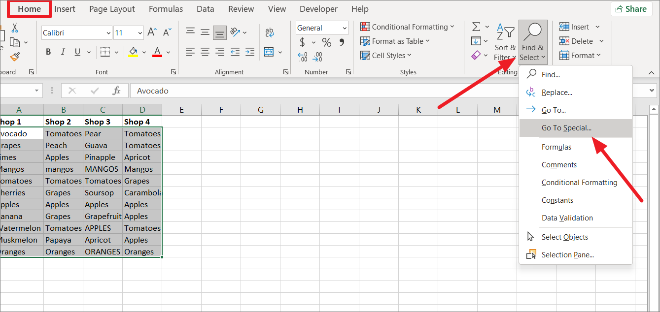
Se você quiser comparar várias colunas e destacar valores diferentes (dados incompatíveis) em cada linha individual, você pode usar o recurso’Ir para especial’no Excel.
Para fazer isso, selecione as colunas que deseja comparar.
Now, you need to specify the comparison column. Os valores das células de outras colunas selecionadas da mesma linha serão comparados com a coluna de comparação para destacar a diferença da célula. Quando você seleciona um intervalo, a célula superior do intervalo é a célula ativa. Na imagem acima, a célula ativa é branca, enquanto as outras células são destacadas em cinza. Aqui, a célula ativa é A3, portanto, a coluna de comparação é A.
Para alterar a coluna de comparação, pressione a tecla Tab para mover a célula ativa da esquerda para a direita ou pressione a tecla Enter para mover de cima para fundo.
Em seguida, clique no botão de menu’Localizar e selecionar’no grupo’Edição’da guia’Início’e selecione’Ir para especial…’.
In the Go To Special dialog box, select’Row differences’and click the’OK’button.
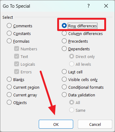
As you can see, all the cell values that are different in the comparison column in each row will be highlighted/selected.
To highlight the selected cells with a color, click the ‘Fill Color’ button on the ribbon and pick a color from the palette.
Compare Two Columns Using VLOOKUP and Extract Matching Data
Sometimes, you may not only want to compare items in one list to the other, but also pull matching data. When comparing columns, there are two types of matches you can use – a partial match or an exact match. This can be done with VLOOKUP or INDEX MATCH function.
The VLOOKUP function is used to search for a specific value in a column and returns a corresponding value from a different column in the same row.
Syntax of VLOOKUP function:
=VLOOKUP(lookup_value,table_array,col_index_num,[range_lookup])
This function consists of 4 parameters or arguments:
lookup_value: This specifies the value that you are searching for in the first column of the given table array. The Lookup value must always be in the left-most column of the search table. table_array: This is the table (range of cells) in which you want to look up a value. This table (search table) can be in the same worksheet or different worksheet, or even a different workbook. col_index_num: This specifies the column number of the table array that has the value you wish to extract. [range_lookup]: This parameter specifies if you want to extract an exact match or an approximate match. It’s either TRUE or FALSE, enter ‘FALSE’ if you want the exact value or enter ‘TRUE’ if you’re OK with the approximate value.
Exact Match
Let’s assume we have two tables with a list of items. In the second, we have a list of items and their prices need to be filled. To do that, we need to compare column A with column D and extract prices for the matching items.
We can use the VLOOKUP function to compare two columns and fetch matching data:
=VLOOKUP(D2,$A$2:$B$13,2,FALSE)
First, enter the formula in cell E2 and then copy the formula down the column by dragging the fill handle.
Where D2 is the value that needs to be searched in the first column of the lookup table. $A$2:$B$13 represents the lookup table where the value will be searched and the corresponding value will be pulled. Here the range is locked into absolute references to prevent the cell reference from changing as the formula is copied down.
The ‘2’ in the formula is the column number of the lookup table with the value you wish to extract. The FALSE parameter is used to find the exact match of D2.
The above formula will search the first column of the range A2:B13 (column A) for the value in D2. An exact match of D2 is found in row 5 of column A, so the corresponding value is extracted from column B (column 2) and returned in E2. When the formula is copied down column E, only the lookup_value value automatically adjusts to D3, D4, etc to search each value of column D in the range A2:B13.
Compare Columns and Pull Matching Data using IFERROR or IFNA functions
In case the lookup_value is not found in the lookup table or the look_up value weren’t exact copies of the values in the look_up table, you would get the #N/A error.
In the below example, lookup_values (D3 and D5) weren’t found in column A and the match type is FALSE (exact), so the formula returns the #N/A error.
This can happen even if there is an extra space, missing space, or a typo in the look_up value. In such cases, you can change the match_type to TRUE which will enable the formula to ignore small errors and look for an approximate match of the values.
If the lookup_value is not found in the table, you can use IFNA or IFERROR function to avoid the #N/A error.
=IFNA(VLOOKUP(D2,$A$2:$B$13,2,FALSE),””)
This formula works the same way as the previous VLOOKUP formula, except the IFNA replaces the error message with a blank. You can also have the formula return a text instead of a blank cell.
Alternatively, you can also use the IFERROR function to remove the error message and return a specified text string. To do that, enter the below formula:
=IFERROR(VLOOKUP(D2,$A$2:$B$13,2,FALSE),”Not Available”)
Enter the above formula in cell E2 and copy it down the column. If the VLOOKUP function returns an #N/A error, then the IFERROR function replaces it with the “Not Available” message as shown below.
Compare Two Columns and Find a Partial Match using Wildcards
In case there are minor differences in the names in the two columns, the TRUE parameter in the VLOOKUP function won’t cover it. For example, if one column has a value called “Google” and the other has “Google LLC”, the above VLOOKUP formula won’t be able to match the columns. However, you can still use the VLOOKUP to partially match columns by adding wildcards to the formula.
The VLOOKUP function allows you to find a partial match on a specified value using wildcard characters. If you want to locate a value that contains the lookup value in any position, add an ampersand sign (&) to join the lookup value with the wildcard character (*). Use ‘$’ signs to make absolute cell references and add the wildcard ‘*’ sign before or after the lookup value.
In the below example, we only have part of a lookup value (Fan) in cell D3. So, to perform a partial match on the given characters, concatenate a wildcard ‘*’ before and after the cell reference.
=VLOOKUP(“*”&D3&”*”,$A$2:$B$13,2,FALSE)
In the above formula, D2 has been enclosed in ‘&’ operators and asterisks “*” to make up for the missing character before and after the lookup value. If List 2 doesn’t have the entire name of the items, the asterisks characters will make up for the missing characters and pull values from the partially matched columns.
For instance, in cell D3 we only have the item named ‘Fan’ but in column A we have ‘Table Fan’. But the asterisks ‘*’ before the D3 made up for the missing ‘Table’ before the lookup value. So, the VLOOKUP function returns the corresponding value ‘31.68’ from column B.
Compare Two Columns using the MATCH Function
If you want to return the position of the matching value in the column instead of the value itself, you can use the MATCH function.
The MATCH function is a built-in function in Excel and its primarily used for locating the relative position of a lookup value in a column or a row.
Syntax of MATCH Function:
=MATCH(lookup_value,lookup_array,[match_type})
Where:
lookup_value – The value you want to look up in a specified range of cells or an array. It can be a numeric value, text value, logical value, or a cell reference that has a value.
lookup_array – The arrays of cells in which you are searching for a value. It must be a single column or a single row.
match_type – It is an optional parameter that can be set to 0,1, or-1 and the default is 1.
0 looks for an exact match, and when it’s not found, returns an error. -1 looks for the smallest value that is greater than or equal to lookup_value when the lookup array is in ascending order. 1 looks for the largest value that is less than or equal to the look_up value when the lookup array is in descending order.
Compare Two Columns and Find the Position of An Exact Match
Let’s assume, we have the following tables where we want to find the position of each value in column D in column A.
=MATCH(D2,$A$2:$A$13,0)
The formula searches for each value of list 2 in list 1 and returns the position of each value.
Display Duplicates or Matching Data using the MATCH function
A combination of MATCH, ISERROR, and IF functions can be used to compare and display duplicates of columns.
For example, we can use the below formula to compare the two columns and display duplicates in the first column:
=IF(ISERROR(MATCH(A2,$B$2:$B$10,0)),””,A2)
Here, the ISERROR function is combined with the IF function to find errors and display text strings or blanks.
The MATCH function searches and returns the position of A2 (in the range B2:B10) as 5. Since it is not an error, the ISERROR function returns FALSE, and the IF function returns the value of A2. In another instance, the MATCH function in C6 returns a #N/A error because the value of A6 is not found in the range B2:B10. Hence, the ISERROR function returns TRUE, and subsequently, the IF function returns the blank.
Display Unique Data using the MATCH function
If you want to compare two columns and display the unique values in each column, you can also do that with the same above formula by simply swapping the last 2 arguments of the IF function.
To display unique values in the first column, enter the below formula:
=IF(ISERROR(MATCH(A2,$B$2:$B$10,0)),A2,””)
The MATCH function searches and returns the position of A2 (in the range B2:B10) as 5. Since the result is not an error, the ISERROR function returns FALSE and the IF function returns the blank space.
The MATCH function in C4 returns a #N/A error because the value of A4 is not found in the range B2:B10. Hence, the ISERROR function returns TRUE, and subsequently, the IF function returns the value of A4.
To display unique values in the second column, enter the below formula:
=IF(ISERROR(MATCH(B2,$A$2:$A$10,0)),B2,””)
The MATCH function looks at and returns the position of B2 (in the range A2:A10) as 5. Since the result is not an error, the ISERROR function returns FALSE and the IF function returns the blank space.
The MATCH function in C4 returns a #N/A error because the value of B4 is not found in the range B2:B10. Hence, the ISERROR function returns TRUE, and subsequently, the IF function returns the value of B4.
Compare Two Columns using INDEX and MATCH Functions
The MATCH function can be combined with the INDEX function to compare and match two columns. Compared to VLOOKUP, the INDEX MATCH is a powerful and versatile formula that can compare two columns and also pull the matching data.
The INDEX function is used to retrieve a value at a specific location in a table or a range. The MATCH function returns the relative position of a value in a column or a row. When combined, the MATCH finds the row or column number (location) of a specific value, and the INDEX function retrieves a value based on that row and column number.
Syntax of INDEX function:
=INDEX(array,row_num,[col_num],) array – The arrays of cells in which you are searching for a value. row_num – It represents the row in the array from which to return a value. If row_num is omitted, column_num is required. column_num – It represents the column in the array from which to return a value. If column_num is omitted, row_num is required.
Example:
To compare the two columns A and D and fetch the price (the matched value) for column D by using INDEX and MATCH:
=INDEX($B$2:$B$13,MATCH(D2,$A$2:$A$13,0))
Enter the formula in cell E2 and copy it down the range E3:E7. Now, let’s see how the formula works:
INDEX function needs a row and column number to retrieve a value. In the above formula, the nested MATCH function finds the row number (position) of the value D2. Then we supply that row number (5) to the INDEX function with a range B2:B13. We specified ‘0’ as the last argument to ignore the column number because we are considering only one column in our array, column B ($B$2:$B$13).
Finally, the INDEX function returns the 5th value in the array B2:B13, which is 24.14.
As you can see, we encountered the #N/A errors in cell E5 because the cell value D5 is not available in column A. To avoid such errors, you can wrap the formula with an IFERROR function.
=IFERROR(INDEX($B$2:$B$13,MATCH(D2,$A$2:$A$13,0)),””)
Using Wildcards
In case there is little difference in the names in the two columns that we are comparing, you can partially match columns by adding wildcards to the formula.
Wildcards can be used in the MATCH function only when match_type is set to ‘0’ and the lookup value is a text string. There are wildcards you can use in the MATCH function: an asterisk (*) and a question mark (?).
Question mark (?) is used to match any single character or letter with the text string. Asterisk (*) is used to match any number of characters with the string.
As you can see below, the names in List 2 are not as complete as in List 1, so using wildcards can make up for the missing characters.
=INDEX($B$2:$B$13,MATCH(“*”&D2&”*”,$A$2:$A$13,0))
In the above formula, D2 has been enclosed in ‘&’ operators and asterisks “*” to make up for the missing character before and after the lookup value. If list 2 doesn’t have the entire name of the items, the asterisks characters will make up for the missing characters and extract values from the partially matched columns.
Compare Two Columns and Find Matches and Differences using VBA Macro
In case you need to compare and match columns often or repeatedly, you can create VBA Macros to automate those tasks. You can use VBA code to create custom user-generated functions to perform tasks and calculations. Here’s how you can do that:
Compare Two Columns Row by Row and Highlight Differences using VBA Code
VBA Macro is the quickest and most effective way to compare two columns in Excel. If you want to compare two columns and highlight the differences between them, follow the instructions:
First, open the workbook that contains the two columns you want to compare.
Then, go to the ‘Developer’ tab and click the ‘Visual Basic’ option from the ribbon or press Alt+F11 keyboard shortcut to open Microsoft Visual Basic for Applications.
This will open Microsoft Visual Basic for Applications in a separate window. In the VBA window, click the ‘Insert’ menu and select the ‘Module’ option. Alternatively, you can just right-click on the ‘Microsoft Excel Objects’ in the navigation bar on the left, click ‘Insert’, and then select ‘Module’ from the sub-menu.
Now, copy and paste the following VBA script into the new module window:
Sub HighlightColumnDifferences() Dim Rg As Range Dim Ws As Worksheet Dim FI As Integer On Error Resume Next SRC: Set Rg=Application.InputBox(“Select Two Columns:”,”Excel”, , , , , , 8) If Rg Is Nothing Then Exit Sub If Rg.Columns.Count <> 2 Then MsgBox”Please Select Two Columns” GoTo SRC End If Set Ws=Rg.Worksheet For FI=1 To Rg.Rows.Count If Not StrComp(Rg.Cells(FI, 1), Rg.Cells(FI, 2), vbBinaryCompare)=0 Then Ws.Range(Rg.Cells(FI, 1), Rg.Cells(FI, 2)).Interior.ColorIndex=6’you can change the color index as you like. End If Next FI End Sub
The above code allows you to compare two columns row by row and highlight the differences between them.
After pasting the script, click ‘File’ and select ‘Save XXXX (filename)’ to save this module as a macro.
The VB script needs to be saved in a macro-enabled file type. Once you click ‘Save’, you will see a prompt box asking whether you want to save this file in a macro-free file or macro-enabled file type.
Click ‘No’ to choose the macro-enabled file type.
In the Save As window, choose the ‘Excel Macro-Enabled Workbook (*.xlsm)’ format from the ‘Save As type’ drop-down.
Then, click the ‘Save’ button to save the VBA macro with the workbook.
Now, you can run the macro to compare columns.
Go back to your Excel worksheet, then he ad to the ‘Developer’ tab in ‘Ribbon’ and select ‘Macros’ or press ALT+F8.
A dialog box named Macro will open up. Under the Macro name, you will see the macro you created. Select the ‘HighlightColumnDifference’ macro and click ‘Run’.
Now, you will see a dialog box for specifying the two columns. Simply select the columns you want to compare and click ‘OK’.
The differences between the two columns will be highlighted with a background color you specified in the code. This VBA code compares columns with case-sensitive and highlights the differences.
Compare Two Columns and Highlight Matching Data (or Duplicates) using VBA Code
If you want to compare two columns and then highlight the matches or duplicates in the second column, you can use the below code.
Open the spreadsheet and press Alt+F11 to open the Microsoft Visual Basic for Applications window. Then, go to ‘Insert’ > ‘Module’ in the Microsoft Visual Basic for Applications window.
Next, copy-paste the below macro code into the new blank Module script:
Sub CompareTwoRanges() Dim xRg, xRgC1, xRgC2, xRgF1, xRgF2 As Range SRg: Set xRgC1=Application.InputBox(“Select the column you want compare according to”,”Excel”, , , , , , 8) If xRgC1 Is Nothing Then Exit Sub If xRgC1.Columns.Count <> 1 Then MsgBox”Please select a single column” GoTo SRg End If SsRg: Set xRgC2=Application.InputBox(“Select the column you want to highlight duplicates in:”,”Excel”, , , , , , 8) If xRgC2 Is Nothing Then Exit Sub If xRgC2.Columns.Count <> 1 Then MsgBox”Please select a single column” GoTo SsRg End If For Each xRgF1 In xRgC1 For Each xRgF2 In xRgC2 If xRgF1.V alue=xRgF2.Value Then xRgF2.Interior.ColorIndex=38′(you can change the color index as you need) End If Next Next End Sub
After pasting the code save the file as a Macro-Enabled Workbook with ‘*.xlsm’ format like we showed you above. Then, close the module and Microsoft Visual Basic for Applications window.
To run the VBA macro, switch to the ‘Developer’ tab and click ‘Macros’ from the Code group.
In the Macro dialog window, select ‘CompareTwoRanges’ and click ‘Run’.
When you see the first pop-up dialog box, select the column that you want to compare duplicate values according to and click ‘OK’.
In the second dialog box, select the column where you want to highlight duplicate values and click ‘OK ’.
As you can see below, the second column is compared against the first column, and duplicates are highlighted in the second column with a background color. This VBA code compares columns with case-sensitive matches.
Compare Two Columns and Extract Matching Data using VBA Code
In case you want to compare two columns row by row and pull the matching values (duplicates) to another column, you can use the below macro code.
Open a blank module in the Microsoft Visual Basic for Applications window as we showed you. Copy and paste the below script to the new blank module:
Sub PullMatches() Dim xRg, xRgC1, xRgC2, xRgF1, xRgF2 As Range Dim xIntSR, xIntER, xIntSC, xIntEC As Integer On Error Resume Next SRg: Set xRgC1=Application.InputBox(“Select first column:”,”Excel”, , , , , , 8) If xRgC1 Is Nothing Then Exit Sub If xRgC1.Columns.Count <> 1 Then MsgBox”Please select single column” GoTo SRg End If SsRg: Set xRgC2=Application.InputBox(“Select the second column:”,”Excel”, , , , , , 8) If xRgC2 Is Nothing Then Exit Sub If xRgC2.Columns.Count <> 1 Then MsgBox”Please select single column” GoTo SsRg End If Set xWs=xRg.Worksheet For FI=1 To xRg.Rows.Count If Not StrComp(xRg.Cells(FI, 1), xRg.Cells(FI, 2), vbBinaryCompare)=0 Then Ws.Range(xRg.Cells(FI, 1), Rg.Cells(FI, 2)).Interior.ColorIndex=8’you can change the color index as you like. End If Next FI End Sub
After pasting the code save the file and close the Microsoft Visual Basic for Applications window. Then, open the Marco dialog window, select the ‘PullMatches’ macro and click ‘Run’.
First, select the first column (left) you want to compare and click ‘OK’.
In the second dialog, select the second column you want to compare and click ‘OK’.
The matches between two columns will be pulled and displayed automatically in the right column of the two columns you selected.
Compare Two Columns and Extract Unique Data using VBA Code
If you want to two compare columns and pull unique values, here’s the below VBA code that can help you.
Open a blank module in the Microsoft Visual Basic for Applications window and copy-paste the below script to the new blank module:
Sub PullUniques() Dim xRg, xRgC1, xRgC2, xFRg1, xFRg2 As Range Dim xIntR, xIntSR, xIntER, xIntSC, xIntEC As Integer Dim xWs As Worksheet On Error Resume Next SRg: Set xRg=Application.InputBox(“Select two columns:”,”Excel”, , , , , , 8) If xRg Is Nothing Then Exit Sub If xRg.Columns.Count <> 2 Then MsgBox”Please select two columns as a range” GoTo SRg End If Set xWs=xRg.Worksheet xIntSC=xRg.Column xIntEC=xRg.Columns.Count + xIntSC-1 xIntSR=xRg.Row xIntER=xRg.Rows.Count + xIntSR-1 Set xRg=xRg.Columns Set xRgC1=xWs.Range(xWs.Cells(xIntSR, xIntSC), xWs.Cells(xIntER, xIntSC)) Set xRgC2=xWs.Range(xWs.Cells(xIntSR, xIntEC), xWs.Cells(xIntER, xIntEC)) xIntR=1 For Each xFRg In xRgC1 If WorksheetFunction.CountIf(xRgC2, xFRg.Value)=0 Then xWs.Cells(xIntER, xIntEC).Offset(xIntR)=xFRg xIntR=xIntR + 1 End If Next xIntR=1 For Each xFRg In xRgC2 If WorksheetFunction.CountIf(xRgC1, xFRg)=0 Then xWs.Cells(xIntER, xIntSC).Offset(xIntR)=xFRg xIntR=xIntR + 1 End If Next End Sub
Then save the file and close the Microsoft Visual Basic for Applications window.
After that, open the Marco dialog window, select the ‘PullUniques’ macro, and click ‘Run’.
In the pop-up window, select the two comparing columns and click ‘OK’.
The Macro compares columns without case sensitivity and lists unique values from the two columns.
That’s it. Now, you know everything about comparing columns in Excel. You can opt for the method that suits you the best.