Bem-vindo de volta a esta série sobre o novo protocolo HTTP/3. Na parte 1, vimos por que exatamente precisamos de HTTP/3 e o subjacente Protocolo QUIC e quais são seus principais novos recursos.
Nesta segunda parte, vamos dar um zoom nas melhorias de desempenho que o QUIC e o HTTP/3 trazem para a web-carregamento da página. No entanto, também seremos um tanto céticos quanto ao impacto que podemos esperar desses novos recursos na prática.
Como veremos, o QUIC e o HTTP/3 realmente têm um grande potencial de desempenho na web, mas principalmente para usuários em redes lentas . Se o seu visitante médio estiver em uma rede rápida com fio ou celular, provavelmente não se beneficiará tanto com os novos protocolos. No entanto, observe que mesmo em países e regiões com uplinks normalmente rápidos, os mais lentos 1% a até 10% de seu público (os chamados 99º ou 90º percentis) ainda têm potencial para ganhar muito. Isso ocorre porque HTTP/3 e QUIC ajudam principalmente a lidar com problemas um tanto incomuns, mas potencialmente de alto impacto, que podem surgir na Internet de hoje.
Esta parte é um pouco mais técnica do que o primeiro, embora transfira a maior parte das coisas realmente profundas para fontes externas, com foco em explicar por que essas coisas são importantes para o desenvolvedor da Web médio.
Esta série é dividida em três partes:
História HTTP/3 e conceitos básicos
Isso é voltado para pessoas que não conhecem HTTP/3 e protocolos em geral, e discute principalmente o básico. Recursos de desempenho HTTP/3 (artigo atual)
Isso é mais aprofundado e técnico. Pessoas que já conhecem o básico podem começar aqui. Opções práticas de implantação de HTTP/3 (em breve!)
Isso explica os desafios envolvidos na implantação e no teste de HTTP/3 por conta própria. Ele detalha como e se você deve alterar suas páginas da web e recursos também. Um manual sobre velocidade
Discutir desempenho e “velocidade” pode se tornar rapidamente complexo, porque muitos aspectos subjacentes contribuem para o carregamento de uma página da web “lentamente”. Como estamos lidando com protocolos de rede aqui, examinaremos principalmente os aspectos da rede, dos quais dois são os mais importantes: latência e largura de banda.
A latência pode ser definida aproximadamente como o tempo que leva para enviar um pacote do ponto A (digamos, o cliente) ao ponto B (o servidor) . É fisicamente limitado pela velocidade da luz ou, praticamente, pela rapidez com que os sinais podem viajar em fios ou ao ar livre. Isso significa que a latência geralmente depende da distância física real entre A e B.
Na terra , isso significa que latências típicas são conceitualmente pequenas, entre cerca de 10 e 200 milissegundos. No entanto, esta é apenas uma maneira: as respostas aos pacotes também precisam voltar. A latência bidirecional geralmente é chamada de tempo de ida e volta (RTT) .
Devido a recursos como o controle de congestionamento (veja abaixo), muitas vezes precisaremos de algumas viagens de ida e volta para carregar até mesmo um único arquivo. Como tal, mesmo latências baixas de menos de 50 milissegundos podem adicionar atrasos consideráveis. Esta é uma das principais razões pelas quais as redes de entrega de conteúdo (CDNs) existem: elas colocam os servidores fisicamente mais próximos do usuário final para reduzir a latência e, portanto, atrasar o máximo possível.
Largura de banda, então , pode ser aproximadamente o número de pacotes que podem ser enviados ao mesmo tempo . Isso é um pouco mais difícil de explicar, porque depende das propriedades físicas do meio (por exemplo, a frequência usada das ondas de rádio), do número de usuários na rede e também dos dispositivos que interconectam diferentes sub-redes (porque eles normalmente só pode processar um determinado número de pacotes por segundo).
Uma metáfora frequentemente usada é a de um cano usado para transportar água. O comprimento do tubo é a latência, enquanto a largura do tubo é a largura de banda. Na Internet, no entanto, normalmente temos uma longa série de tubos conectados , alguns dos quais podem ser mais largos do que outros (levando aos chamados gargalos nos links mais estreitos). Como tal, a largura de banda ponta a ponta entre os pontos A e B é frequentemente limitada pelas subseções mais lentas.
Embora um entendimento perfeito desses conceitos não seja necessário para o restante deste post, ter um uma definição de alto nível seria boa. Para obter mais informações, recomendo verificar o excelente capítulo sobre latência e largura de banda de Ilya Grigorik em seu livro High Performance Rede do navegador.
Controle de congestionamento
Um aspecto do desempenho é sobre como eficientemente um protocolo de transporte pode usar a largura de banda total (física) de uma rede (ou seja, aproximadamente, quantos pacotes por segundo podem ser enviado ou recebido). Isso, por sua vez, afeta a rapidez com que os recursos de uma página podem ser baixados. Alguns afirmam que o QUIC de alguma forma faz isso muito melhor do que o TCP, mas isso não é verdade.
Você sabia?
Uma conexão TCP, por exemplo, não apenas começa a enviar dados com largura de banda total, porque isso pode acabar sobrecarregando (ou congestionando) a rede. Isso porque, como dissemos, cada link de rede possui apenas uma determinada quantidade de dados que pode (fisicamente) processar a cada segundo. Dê mais um tempo e não haverá outra opção senão descartar os pacotes em excesso, levando à perda de pacotes .
Conforme discutido em parte 1 , para um protocolo confiável como o TCP, a única maneira de se recuperar da perda de pacotes é retransmitindo uma nova cópia dos dados , o que leva uma viagem de ida e volta. Especialmente em redes de alta latência (digamos, com um RTT de mais de 50 milissegundos), a perda de pacotes pode afetar seriamente o desempenho.
Outro problema é que não sabemos de antemão quanto é o máximo largura de banda será. Muitas vezes depende de um gargalo em algum lugar na conexão ponta a ponta, mas não podemos prever ou saber onde isso estará. A Internet também não tem mecanismos (ainda) para sinalizar capacidades de link de volta aos terminais.
Além disso, mesmo se soubéssemos a largura de banda física disponível, isso não significaria que poderíamos usar tudo isso nós mesmos. Vários usuários estão normalmente ativos em uma rede ao mesmo tempo, cada um dos quais precisa de uma parte justa da largura de banda disponível.
Dessa forma, uma conexão não sabe quanta largura de banda pode usar antecipadamente de maneira segura ou justa, e essa largura de banda pode mudar conforme os usuários entram, saem e usam a rede. Para resolver este problema, o TCP tentará constantemente descobrir a largura de banda disponível ao longo do tempo usando um mecanismo chamado controle de congestionamento .
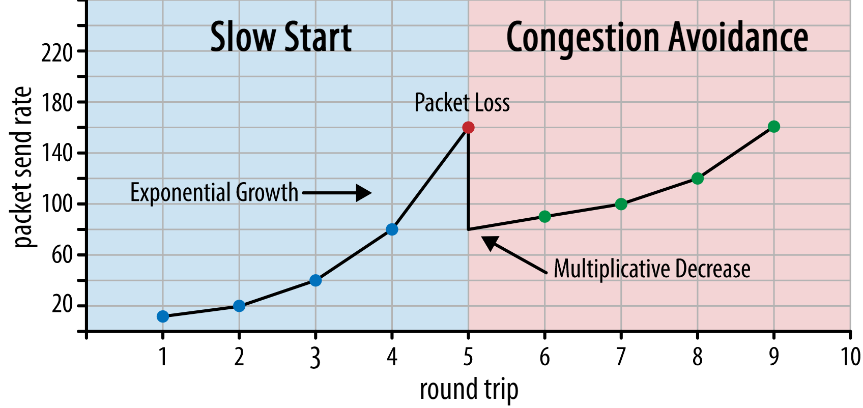
No início da conexão, ele envia apenas alguns pacotes (na prática, variando entre 10 e 100 pacotes, ou cerca de 14 e 140 KB de dados) e espera uma viagem de ida e volta até que o receptor envie as confirmações desses pacotes. Se todos forem confirmados, isso significa que a rede pode lidar com essa taxa de envio e podemos tentar repetir o processo, mas com mais dados (na prática, a taxa de envio geralmente dobra a cada iteração).
Dessa forma, a taxa de envio continua a crescer até que alguns pacotes não sejam reconhecidos (o que indica perda de pacotes e congestionamento da rede). Esta primeira fase é normalmente chamada de “início lento”. Ao detectar a perda de pacotes, o TCP reduz a taxa de envio e (depois de um tempo) começa a aumentar a taxa de envio novamente, embora em incrementos (muito) menores. Essa lógica de redução e crescimento é repetida para cada perda de pacote posteriormente. Eventualmente, isso significa que o TCP tentará constantemente alcançar sua divisão de largura de banda justa e ideal. Esse mecanismo é ilustrado na figura 1.
Esta é uma explicação extremamente simplificada do controle de congestionamento. Na prática, muitos outros fatores estão em jogo, como bufferbloat , o flutuação de RTTs devido ao congestionamento , e o fato de que vários remetentes simultâneos precisam obter seus compartimento justo da largura de banda . Como tal, existem muitos algoritmos de controle de congestionamento diferentes, e muitos ainda estão sendo inventados hoje, sem nenhum desempenho ideal em todas as situações.
Embora o controle de congestionamento do TCP o torne robusto, também significa que leva um tempo para alcançar taxas de envio ideais , dependendo do RTT e da largura de banda real disponível. Para carregamento de página da web, essa abordagem de início lento também pode afetar métricas como a primeira pintura com conteúdo, porque apenas uma pequena quantidade de dados (dezenas a algumas centenas de KB) pode ser transferida nas primeiras viagens de ida e volta. (Você deve ter ouvido a recomendação para manter seus dados críticos com menos de 14 KB .)
A escolha de uma abordagem mais agressiva pode levar a melhores resultados em redes de alta largura de banda e alta latência, especialmente se você não se importar com a perda ocasional de pacotes. Foi aqui que vi novamente muitas interpretações errôneas sobre como o QUIC funciona.
Conforme discutido em parte 1 , QUIC, em teoria, sofre menos com a perda de pacotes (e o bloqueio de ponta de linha (HOL) relacionado) porque trata a perda de pacotes em cada recurso fluxo de bytes de forma independente. Além disso, o QUIC é executado no User Datagram Protocol (UDP), que, ao contrário do TCP, não possui um recurso de controle de congestionamento embutido; ele permite que você tente enviar na taxa que quiser e não retransmite dados perdidos.
Isso levou a muitos artigos alegando que o QUIC também não usa controle de congestionamento, que o QUIC pode, em vez disso, começar a enviar dados a uma taxa muito mais alta sobre UDP (contando com a remoção do bloqueio HOL para lidar com a perda de pacotes), é por isso que o QUIC é muito mais rápido do que o TCP.
Na realidade, nada poderia estar mais longe da verdade : O QUIC na verdade usa técnicas de gerenciamento de largura de banda muito semelhantes ao TCP . Ele também começa com uma taxa de envio mais baixa e aumenta com o tempo, usando os reconhecimentos como um mecanismo-chave para medir a capacidade da rede. Isso ocorre (entre outras razões) porque o QUIC precisa ser confiável para ser útil para algo como HTTP, porque precisa ser justo com outras conexões QUIC (e TCP!) E porque sua remoção de bloqueio de HOL não na verdade, ajuda muito bem contra a perda de pacotes (como veremos a seguir).
No entanto, isso não significa que o QUIC não possa ser (um pouco) mais inteligente sobre como gerencia a largura de banda do que o TCP. Isso ocorre principalmente porque o QUIC é mais flexível e fácil de evoluir do que o TCP . Como dissemos, os algoritmos de controle de congestionamento ainda estão em forte evolução hoje e provavelmente precisaremos, por exemplo, ajuste as coisas para obter o máximo do 5G .
No entanto, o TCP é normalmente implementado no kernel do sistema operacional (OS’), um ambiente seguro e mais restrito, que para a maioria dos sistemas operacionais não é nem mesmo de código aberto. Como tal, o ajuste da lógica de congestionamento geralmente é feito apenas por alguns poucos desenvolvedores selecionados, e a evolução é lenta.
Em contraste, a maioria das implementações do QUIC estão sendo feitas no”espaço do usuário”(onde normalmente executamos aplicativos nativos ) e são feitos de código aberto , explicitamente para encorajar a experimentação por um grupo muito maior de desenvolvedores (como já mostrado , por exemplo, pelo Facebook ).
Outro exemplo concreto é o frequência de confirmação atrasada proposta de extensão para QUIC. Embora, por padrão, o QUIC envie uma confirmação para cada 2 pacotes recebidos, esta extensão permite que os terminais reconheçam, por exemplo, a cada 10 pacotes. Foi demonstrado que isso oferece benefícios de grande velocidade em redes de satélite e de largura de banda muito alta, porque a sobrecarga de transmissão dos pacotes de confirmação é reduzida. Adicionar tal extensão para TCP levaria muito tempo para ser adotado, enquanto para QUIC é muito mais fácil de implantar.
Assim, podemos esperar que a flexibilidade do QUIC levará a mais experimentação e melhor controle de congestionamento algoritmos ao longo do tempo, que por sua vez também poderiam ser portados para o TCP para melhorá-lo também.
Você sabia?
O QUIC Recovery RFC 9002 especifica o uso do algoritmo de controle de congestionamento NewReno. Embora essa abordagem seja robusta, ela também está um pouco desatualizada e não é mais usada extensivamente na prática. Então, por que está no QUIC RFC? A primeira razão é que, quando o QUIC foi iniciado, NewReno era o algoritmo de controle de congestionamento mais recente, ele próprio padronizado. Algoritmos mais avançados, como BBR e CUBIC, ainda não estão padronizados ou apenas recentemente se tornaram RFCs.
A segunda razão é que NewReno é uma configuração relativamente simples. Como os algoritmos precisam de alguns ajustes para lidar com as diferenças do QUIC em relação ao TCP, é mais fácil explicar essas mudanças em um algoritmo mais simples. Como tal, o RFC 9002 deve ser lido mais como “como adaptar um algoritmo de controle de congestionamento ao QUIC”, em vez de “isso é o que você deve usar para o QUIC”. Na verdade, a maioria das implementações de QUIC de nível de produção fez implementações personalizadas de Cubic e BBR .
Vale a pena repetir os algoritmos de controle de congestionamento não são específicos de TCP ou QUIC ; eles podem ser usados por qualquer um dos protocolos e espera-se que os avanços no QUIC eventualmente também encontrem seu caminho para as pilhas TCP.
Você sabia?
Observe que, ao lado do controle de congestionamento está um conceito relacionado chamado controle de fluxo . Esses dois recursos são frequentemente confundidos no TCP, porque ambos usam a “janela TCP” , embora na verdade existam duas janelas: a janela de congestionamento e a janela de recepção do TCP. O controle de fluxo, no entanto, entra em ação muito menos para o caso de uso de carregamento de página da web no qual estamos interessados, portanto, vamos ignorá-lo aqui. Mais em profundidade as informações estão disponíveis .
O que isso tudo significa?
O QUIC ainda está sujeito às leis da física e à necessidade de ser gentil com outros remetentes na Internet. Isso significa que ele não fará o download magicamente dos recursos do seu site com muito mais rapidez do que o TCP. No entanto, a flexibilidade do QUIC significa que experimentar novos algoritmos de controle de congestionamento se tornará mais fácil, o que deve melhorar as coisas no futuro para TCP e QUIC.
Configuração da conexão 0-RTT
Um segundo aspecto de desempenho é sobre quantas viagens de ida e volta leva antes que você possa enviar dados HTTP úteis (por exemplo, recursos de página) em uma nova conexão. Alguns afirmam que o QUIC é duas a três viagens de ida e volta mais rápido do que TCP + TLS, mas veremos que é realmente apenas um.
Você sabia?
Como dissemos na parte 1 , uma conexão normalmente funciona um (TCP) ou dois (TCP + TLS) handshakes antes que as solicitações e respostas HTTP possam ser trocadas. Esses handshakes trocam parâmetros iniciais que o cliente e o servidor precisam saber para, por exemplo, criptografar os dados.
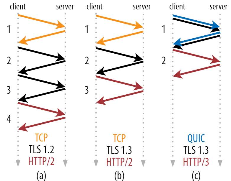
Como você pode ver na figura 2 abaixo, cada handshake individual leva pelo menos uma viagem de ida e volta para concluir (TCP + TLS 1.3, (b)) e às vezes dois (TLS 1.2 e anterior (a)). Isso é ineficiente, porque precisamos de pelo menos duas viagens de ida e volta de tempo de espera do handshake (sobrecarga) antes de enviarmos nossa primeira solicitação HTTP, o que significa esperar pelo menos três viagens de ida e volta para os primeiros dados de resposta HTTP ( a seta vermelha de retorno) para entrar. Em redes lentas, isso pode significar uma sobrecarga de 100 a 200 milissegundos.
Você pode estar se perguntando por que o handshake TCP + TLS não pode ser simplesmente combinado, feito na mesma viagem de ida e volta. Embora isso seja conceitualmente possível (o QUIC faz exatamente isso), inicialmente as coisas não foram projetadas assim, porque precisamos ser capazes de use TCP com e sem TLS na parte superior . Em outras palavras, o TCP simplesmente não suporta o envio de coisas não TCP durante o handshake. Houve esforços para adicionar isso com a extensão TCP Fast Open; no entanto, conforme discutido na parte 1 , acabou sendo difícil de implantar em escala .
Felizmente, o QUIC foi projetado com o TLS em mente desde o início e, como tal, combina o transporte e os apertos de mão criptográficos em um único mecanismo. Isso significa que o handshake QUIC levará apenas uma viagem de ida e volta no total, que é uma viagem de ida e volta a menos do que TCP + TLS 1.3 (consulte a figura 2c acima).
Você pode estar confuso, porque você’Provavelmente li que o QUIC é duas ou até três viagens de ida e volta mais rápidas do que o TCP, não apenas uma. Isso porque a maioria dos artigos considera apenas o pior caso (TCP + TLS 1.2, (a)), sem mencionar que o TCP + TLS 1.3 moderno também “apenas” faz duas viagens de ida e volta ((b) raramente é mostrado). Embora um aumento de velocidade em uma viagem de ida e volta seja bom, não é incrível. Especialmente em redes rápidas (digamos, menos de um RTT de 50 milissegundos), isso será quase imperceptível , embora redes lentas e conexões com servidores distantes lucrem um pouco mais.
Em seguida, você deve estar se perguntando por que precisamos esperar pelo (s) handshake (s). Por que não podemos enviar uma solicitação HTTP na primeira viagem de ida e volta? Isso ocorre principalmente porque, se o fizéssemos, a primeira solicitação seria enviada não criptografada , podendo ser lida por qualquer bisbilhoteiro na transmissão, o que obviamente não é ótimo para privacidade e segurança. Assim, precisamos aguardar a conclusão do handshake criptográfico antes de enviar a primeira solicitação HTTP. Ou não?
É aqui que um truque inteligente é usado na prática. Sabemos que os usuários costumam revisitar as páginas da web logo após sua primeira visita. Como tal, podemos usar a conexão criptografada inicial para inicializar uma segunda conexão no futuro. Simplificando, em algum momento durante sua vida útil, a primeira conexão é usada para comunicar com segurança novos parâmetros criptográficos entre o cliente e o servidor. Esses parâmetros podem então ser usados para criptografar a segunda conexão desde o início, sem ter que esperar a conclusão do handshake TLS completo. Essa abordagem é chamada de “retomada da sessão”.
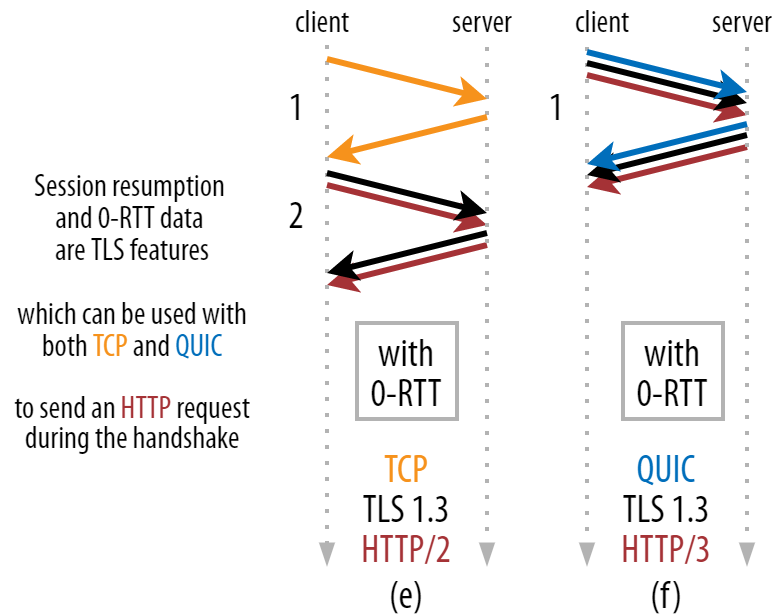
Ela permite uma otimização poderosa: agora podemos enviar com segurança nossa primeira solicitação HTTP junto com o handshake QUIC/TLS, economizando outra viagem de ida e volta ! Quanto ao TLS 1.3, isso remove efetivamente o tempo de espera do handshake TLS. Este método é frequentemente chamado de 0-RTT (embora, é claro, ainda leve uma viagem de ida e volta para os dados de resposta HTTP começarem a chegar).
Tanto a retomada da sessão quanto 0-RTT são, novamente, coisas que Já vi muitas vezes explicadas erroneamente como sendo recursos específicos do QUIC. Na realidade, esses são recursos TLS que já estavam presentes de alguma forma no TLS 1.2 e agora estão totalmente desenvolvidos em TLS 1.3 .
Em outras palavras, como você pode ver na figura 3 abaixo, podemos obter os benefícios de desempenho desses recursos sobre o TCP (e, portanto, também HTTP/2 e até HTTP/1.1) ! Vemos que, mesmo com 0-RTT, o QUIC ainda é apenas uma viagem de ida e volta mais rápido do que uma pilha TCP + TLS 1.3 com funcionamento ideal. A afirmação de que o QUIC é três viagens de ida e volta mais rápido vem da comparação da figura 2 (a) com a figura 3 (f), o que, como vimos, não é realmente justo.
O pior parte é que, ao usar 0-RTT, o QUIC não consegue nem mesmo usar essa viagem de ida e volta ganha muito bem devido à segurança. Para entender isso, precisamos entender um dos motivos pelos quais existe o handshake TCP. Em primeiro lugar, permite que o cliente tenha certeza de que o servidor está realmente disponível no endereço IP fornecido antes de enviar quaisquer dados de camada superior.
Em segundo lugar, e o mais importante aqui, permite que o servidor certifique-se de que o cliente que está abrindo a conexão é realmente quem e onde ele diz que está antes de enviar os dados. Se você se lembra de como definimos uma conexão com a 4-tupla na parte 1 , você saberá que o cliente é identificado principalmente por seu endereço IP. E este é o problema: endereços IP podem ser falsificados !
Suponha que um invasor solicite um arquivo muito grande via HTTP sobre QUIC 0-RTT. No entanto, eles falsificam seu endereço IP, fazendo parecer que a solicitação 0-RTT veio do computador da vítima. Isso é mostrado na figura 4 abaixo. O servidor QUIC não tem como detectar se o IP foi falsificado, porque este é o (s) primeiro (s) pacote (s) que ele está vendo desse cliente.
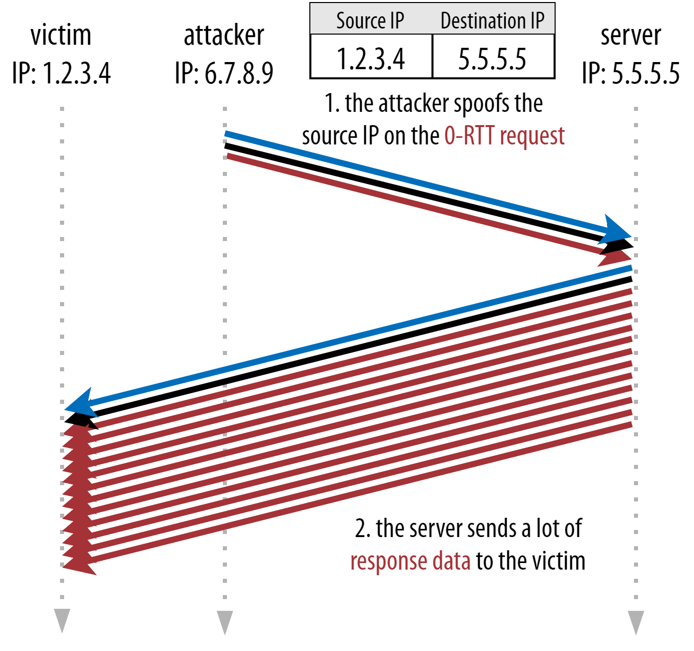
Se o servidor simplesmente começar a enviar o arquivo grande de volta para o IP falsificado, ele pode acabar sobrecarregando a largura de banda da rede da vítima (especialmente se o invasor fizer muitas dessas solicitações falsas em paralelo). Observe que a resposta QUIC seria descartada pela vítima, porque ela não espera dados de entrada, mas isso não importa: a rede deles ainda precisa processar os pacotes!
Isso é chamado de reflexão ou amplificação, ataque , e é uma forma significativa de hackers executam ataques distribuídos de negação de serviço (DDoS). Observe que isso não acontece quando 0-RTT sobre TCP + TLS está sendo usado, precisamente porque o handshake TCP precisa ser concluído antes que a solicitação 0-RTT seja enviada junto com o handshake TLS.
Como tal, o QUIC deve ser conservador ao responder às solicitações 0-RTT, limitando a quantidade de dados que ele envia em resposta até que o cliente tenha sido verificado para ser um cliente real e não uma vítima. Para QUIC, esse valor de dados foi definido como três vezes o valor recebido do cliente .
Em outras palavras, o QUIC tem um”fator de amplificação”máximo de três, que foi determinado como uma compensação aceitável entre a utilidade do desempenho e o risco de segurança (especialmente em comparação com alguns incidentes que tiveram um fator de amplificação de mais de 51.000 vezes ). Como o cliente normalmente envia primeiro apenas um a dois pacotes, a resposta 0-RTT do servidor QUIC será limitada a apenas 4 a 6 KB (incluindo outra sobrecarga de QUIC e TLS!), Que é um pouco menor que impressionante.
Além disso, outros problemas de segurança podem levar a, por exemplo, “ataques de repetição”, que limitam o tipo de solicitação HTTP que você pode fazer. Por exemplo, o Cloudflare permite apenas solicitações HTTP GET sem parâmetros de consulta em 0-RTT. Isso limita a utilidade do 0-RTT ainda mais.
Felizmente, o QUIC tem opções para torná-lo um pouco melhor. Por exemplo, o servidor pode verificar se o 0-RTT vem de um IP com o qual ele teve uma conexão válida antes . No entanto, isso só funciona se o cliente permanecer na mesma rede (limitando um pouco o recurso de migração de conexão do QUIC). E mesmo se funcionar, a resposta do QUIC ainda é limitada pela lógica de início lento do controlador de congestionamento que discutimos acima ; portanto, não há nenhum aumento de velocidade extra massivo além da viagem de ida e volta salva.
Você sabia?
É interessante notar que o limite de amplificação de três vezes do QUIC também conta para seu processo de handshake normal não-0-RTT na figura 2c. Isso pode ser um problema se, por exemplo, o certificado TLS é muito grande para caber em 4 a 6 KB. Nesse caso, ele teria que ser dividido, com o segundo bloco tendo que esperar pelo envio da segunda viagem de ida e volta (após as confirmações dos primeiros pacotes, indicando que o IP do cliente não foi falsificado). Nesse caso, o handshake do QUIC ainda pode levar a duas viagens de ida e volta , igual a TCP + TLS! É por isso que, para o QUIC, técnicas como compactação de certificado serão extras importante.
Você sabia?
Pode ser que certas configurações avançadas sejam capazes de mitigar esses problemas o suficiente para tornar o 0-RTT mais útil. Por exemplo, o servidor poderia lembrar quanta largura de banda um cliente tinha disponível na última vez em que foi visto, tornando-o menos limitado pelo início lento do controle de congestionamento para reconectar clientes (não falsificados). Isso foi investigado na academia e existe até um extensão proposta no QUIC para fazer isso. Várias empresas já fazem esse tipo de coisa para acelerar o TCP também.
Outra opção seria fazer com que os clientes enviassem mais de um ou dois pacotes (por exemplo, enviando 7 mais pacotes com preenchimento), então o limite de três vezes se traduz em uma resposta mais interessante de 12 a 14 KB, mesmo após a migração da conexão. Escrevi sobre isso em um de meus artigos .
Por fim, os servidores QUIC (com comportamento inadequado) também podem aumentar intencionalmente o limite de três vezes se acharem que é seguro fazer isso ou se não se importarem com os possíveis problemas de segurança (afinal, não há protocolopolicial que evita isso).
O que significa tudo isso?
Configuração de conexão mais rápida do QUIC com 0-RTT é realmente mais uma microotimização do que um novo recurso revolucionário. Comparado com uma configuração TCP + TLS 1.3 de última geração, ele economizaria no máximo uma viagem de ida e volta. A quantidade de dados que realmente podem ser enviados na primeira viagem de ida e volta é limitada por uma série de considerações de segurança.
Dessa forma, esse recurso vai brilhar principalmente se seus usuários estiverem em redes com latência muito alta (digamos, redes de satélite com RTTs de mais de 200 milissegundos) ou se você normalmente não envia muitos dados. Alguns exemplos do último são sites com muito cache, bem como aplicativos de página única que buscam periodicamente pequenas atualizações por meio de APIs e outros protocolos, como DNS-over-QUIC . Um dos motivos pelos quais o Google obteve resultados de 0-RTT muito bons para QUIC foi que ele o testou em sua página de pesquisa já altamente otimizada, onde as respostas das consultas são muito pequenas.
Em outros casos, você ganhará apenas algumas dezenas de milissegundos no máximo , menos ainda se você já estiver usando um CDN (o que deve ser feito se você se preocupa com o desempenho!).
Migração de conexão
Um terceiro recurso de desempenho torna o QUIC mais rápido durante a transferência entre redes, por mantendo as conexões existentes intactas . Embora isso realmente funcione, esse tipo de mudança de rede não acontece com tanta frequência e as conexões ainda precisam redefinir suas taxas de envio.
Conforme discutido em parte 1 , os IDs de conexão (CIDs) do QUIC permitem que ele execute a migração de conexão ao trocar de rede . Ilustramos isso com um cliente migrando de uma rede Wi-Fi para 4G durante o download de um arquivo grande. No TCP, esse download pode ter que ser abortado, enquanto no QUIC ele pode continuar.
Primeiro, entretanto, considere a frequência com que esse tipo de cenário realmente acontece. Você pode pensar que isso também ocorre ao mover-se entre pontos de acesso Wi-Fi dentro de um edifício ou entre torres de celular enquanto estiver na estrada. Nessas configurações, no entanto (se forem feitas corretamente), seu dispositivo normalmente manterá seu IP intacto, porque a transição entre as estações base sem fio é feita em uma camada de protocolo inferior. As such, it occurs only when you move between completely different networks, which I’d say doesn’t happen all that often.
Secondly, we can ask whether this also works for other use cases besides large file downloads and live video conferencing and streaming. If you’re loading a web page at the exact moment of switching networks, you might have to re-request some of the (later) resources indeed.
However, loading a page typically takes in the order of seconds, so that coinciding with a network switch is also not going to be very common. Additionally, for use cases where this is a pressing concern, other mitigations are typically already in place. For example, servers offering large file downloads can support HTTP range requests to allow resumable downloads.
Because there is typically some overlap time between network 1 dropping off and network 2 becoming available, video apps can open multiple connections (1 per network), syncing them before the old network goes away completely. The user will still notice the switch, but it won’t drop the video feed entirely.
Thirdly, there is no guarantee that the new network will have as much bandwidth available as the old one. As such, even though the conceptual connection is kept intact, the QUIC server cannot just keep sending data at high speeds. Instead, to avoid overloading the new network, it needs to reset (or at least lower) the send rate and start again in the congestion controller’s slow-start phase.
Because this initial send rate is typically too low to really support things such as video streaming, you will see some quality loss or hiccups, even on QUIC. In a way, connection migration is more about preventing connection context churn and overhead on the server than about improving performance.
Did You Know?
Note that, as discussed for 0-RTT above, we can devise some advanced techniques to improve connection migration. For example, we can, again, try to remember how much bandwidth was available on a given network last time and attempt to ramp up faster to that level for a new migration. Additionally, we could envision not simply switching between networks, but using both at the same time. This concept is called multipath, and we discuss it in more detail below.
So far, we have mainly talked about active connection migration, where users move between different networks. There are, however, also cases of passive connection migration, where a certain network itself changes parameters. A good example of this is network address translation (NAT) rebinding. While a full discussion of NAT is out of the scope of this article, it mainly means that the connection’s port numbers can change at any given time, without warning. This also happens much more often for UDP than TCP in most routers.
If this occurs, the QUIC CID will not change, and most implementations will assume that the user is still on the same physical network and will thus not reset the congestion window or other parameters. QUIC also includes some features such as PINGs and timeout indicators to prevent this from happening, because this typically occurs for long-idle connections.
We discussed in part 1 that QUIC doesn’t just use a single CID for security reasons. Instead, it changes CIDs when performing active migration. In practice, it’s even more complicated, because both client and server have separate lists of CIDs, (called source and destination CIDs in the QUIC RFC). This is illustrated in figure 5 below.
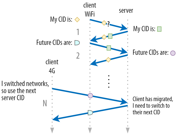
This is done to allow each endpoint to choose its own CID format and contents, which in turn is crucial to allowing advanced routing and load-balancing logic. With connection migration, load balancers can no longer just look at the 4-tuple to identify a connection and send it to the correct back-end server. However, if all QUIC connections were to use random CIDs, this would heavily increase memory requirements at the load balancer, because it would need to store mappings of CIDs to back-end servers. Additionally, this would still not work with connection migration, as the CIDs change to new random values.
As such, it’s important that QUIC back-end servers deployed behind a load balancer have a predictable format of their CIDs, so that the load balancer can derive the correct back-end server from the CID, even after migration. Some options for doing this are described in the IETF’s proposed document. To make this all possible, the servers need to be able to choose their own CID, which wouldn’t be possible if the connection initiator (which, for QUIC, is always the client) chose the CID. This is why there is a split between client and server CIDs in QUIC.
What does it all mean?
Thus, connection migration is a situational feature. Initial tests by Google, for example, show low percentage improvements for its use cases. Many QUIC implementations don’t yet implement this feature. Even those that do will typically limit it to mobile clients and apps and not their desktop equivalents. Some people are even of the opinion that the feature isn’t needed, because opening a new connection with 0-RTT should have similar performance properties in most cases.
Still, depending on your use case or user profile, it could have a large impact. If your website or app is most often used while on the move (say, something like Uber or Google Maps), then you’d probably benefit more than if your users were typically sitting behind a desk. Similarly, if you’re focusing on constant interaction (be it video chat, collaborative editing, or gaming), then your worst-case scenarios should improve more than if you have a news website.
Head-of-Line Blocking Removal
The fourth performance feature is intended to make QUIC faster on networks with a high amount of packet loss by mitigating the head-of-line (HoL) blocking problem. While this is true in theory, we will see that in practice this will probably only provide minor benefits for web-page loading performance.
To understand this, though, we first need to take a detour and talk about stream prioritization and multiplexing.
Stream Prioritization
As discussed in part 1, a single TCP packet loss can delay data for multiple in-transit resources because TCP’s bytestream abstraction considers all data to be part of a single file. QUIC, on the other hand, is intimately aware that there are multiple concurrent bytestreams and can handle loss on a per-stream basis. However, as we’ve also seen, these streams are not truly transmitting data in parallel: Rather, the stream data is multiplexed onto a single connection. This multiplexing can happen in many different ways.
For example, for streams A, B, and C, we might see a packet sequence of ABCABCABCABCABCABCABCABC, where we change the active stream in each packet (let’s call this round-robin). However, we might also see the opposite pattern of AAAAAAAABBBBBBBBCCCCCCCC, where each stream is completed in full before starting the next one (let’s call this sequential). Of course, many other options are possible in between these extremes (AAAABBCAAAAABBC…, AABBCCAABBCC…, ABABABCCCC…, etc.). The multiplexing scheme is dynamic and driven by an HTTP-level feature called stream prioritization (discussed later in this article).
As it turns out, which multiplexing scheme you choose can have a huge impact on website loading performance. You can see this in the video below, courtesy of Cloudflare, as every browser uses a different multiplexer. The reasons why are quite complex, and I’ve written several academic papers on the topic, as well as talked about it in a conference. Patrick Meenan, of Webpagetest fame, even has a three-hour tutorial on just this topic.
 Stream multiplexing differences can have a large impact on website loading in different browsers. (Large preview)
Luckily, we can explain the basics relatively easily. As you may know, some resources can be render blocking. This is the case for CSS files and for some JavaScript in the HTML head element. While these files are loading, the browser cannot paint the page (or, for example, execute new JavaScript).
What’s more, CSS and JavaScript files need to be downloaded in full in order to be used (although they can often be incrementally parsed and compiled). As such, these resources need to be loaded as soon as possible, with the highest priority. Let’s contemplate what would happen if A, B, and C were all render-blocking resources.
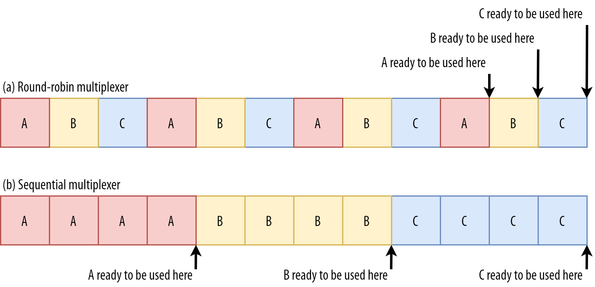
If we use a round-robin multiplexer (the top row in figure 6), we would actually delay each resource’s total completion time, because they all need to share bandwidth with the others. Since we can only use them after they are fully loaded, this incurs a significant delay. However, if we multiplex them sequentially (the bottom row in figure 6), we would see that A and B complete much earlier (and can be used by the browser), while not actually delaying C’s completion time.
However, that doesn’t mean that sequential multiplexing is always the best, because some (mostly non-render-blocking) resources (such as HTML and progressive JPEGs) can actually be processed and used incrementally. In those (and some other) cases, it makes sense to use the first option (or at least something in between).
Still, for most web-page resources, it turns out that sequential multiplexing performs best. This is, for example, what Google Chrome is doing in the video above, while Internet Explorer is using the worst-case round-robin multiplexer.
Packet Loss Resilience
Now that we know that all streams aren’t always active at the same time and that they can be multiplexed in different ways, we can consider what happens if we have packet loss. As explained in part 1, if one QUIC stream experiences packet loss, then other active streams can still be used (whereas, in TCP, all would be paused).
However, as we’ve just seen, having many concurrent active streams is typically not optimal for web performance, because it can delay some critical (render-blocking) resources, even without packet loss! We’d rather have just one or two active at the same time, using a sequential multiplexer. However, this reduces the impact of QUIC’s HoL blocking removal.
Imagine, for example, that the sender could transmit 12 packets at a given time (see figure 7 below) — remember that this is limited by the congestion controller). If we fill all 12 of those packets with data for stream A (because it’s high priority and render-blocking — think main.js), then we would have only one active stream in that 12-packet window.
If one of those packets were to be lost, then QUIC would still end up fully HoL blocked because there would simply be no other streams it could process besides A: All of the data is for A, and so everything would still have to wait (we don’t have B or C data to process), similar to TCP.
We see that we have a kind of contradiction: Sequential multiplexing (AAAABBBBCCCC) is typically better for web performance, but it doesn’t allow us to take much advantage of QUIC’s HoL blocking removal. Round-robin multiplexing (ABCABCABCABC) would be better against HoL blocking, but worse for web performance. As such, one best practice or optimization can end up undoing another.
And it gets worse. Up until now, we’ve sort of assumed that individual packets get lost one at a time. However, this isn’t always true, because packet loss on the Internet is often “bursty”, meaning that multiple packets often get lost at the same time.
As discussed above, an important reason for packet loss is that a network is overloaded with too much data, having to drop excess packets. This is why the congestion controller starts sending slowly. However, it then keeps growing its send rate until… there is packet loss!
Put differently, the mechanism that’s intended to prevent overloading the network actually overloads the network (albeit in a controlled fashion). On most networks, that occurs after quite a while, when the send rate has increased to hundreds of packets per round trip. When those reach the limit of the network, several of them are typically dropped together, leading to the bursty loss patterns.
Did You Know?
This is one of the reasons why we wanted to move to using a single (TCP) connection with HTTP/2, rather than the 6 to 30 connections with HTTP/1.1. Because each individual connection ramps up its send rate in pretty much the same way, HTTP/1.1 could get a good speed-up at the start, but the connections could actually start causing massive packet loss for each other as they caused the network to become overloaded.
At the time, Chromium developers speculated that this behaviour caused most of the packet loss seen on the Internet. This is also one of the reasons why BBR has become an often used congestion-control algorithm, because it uses fluctuations in observed RTTs, rather than packet loss, to assess available bandwidth.
Did You Know?
Other causes of packet loss can lead to fewer or individual packets becoming lost (or unusable), especially on wireless networks. There, however, the losses are often detected at lower protocol layers and solved between two local entities (say, the smartphone and the 4G cellular tower), rather than by retransmissions between the client and the server. These usually don’t lead to real end-to-end packet loss, but rather show up as variations in packet latency (or “jitter”) and reordered packet arrivals.
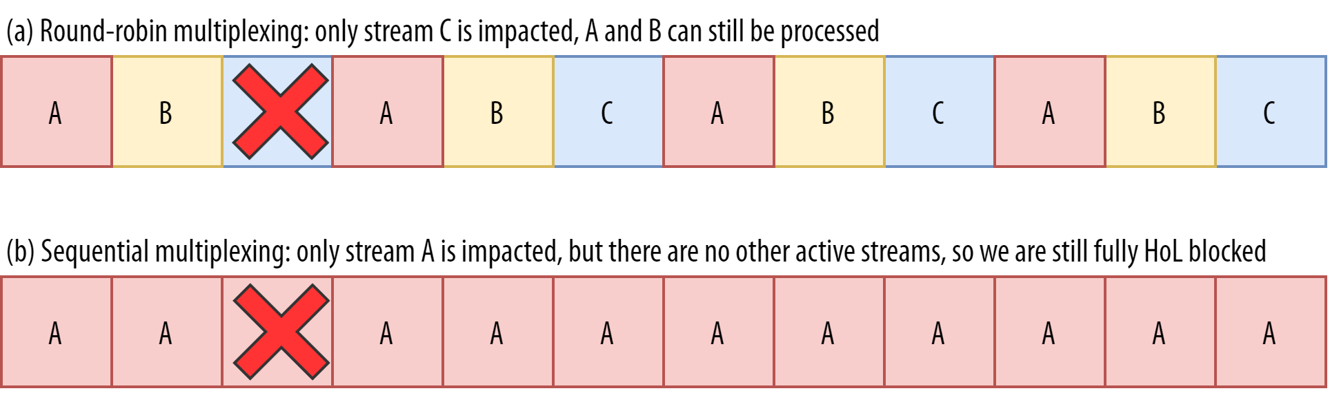
So, let’s say we are using a per-packet round-robin multiplexer (ABCABCABCABCABCABCABCABC…) to get the most out of HoL blocking removal, and we get a bursty loss of just 4 packets. We see that this will always impact all 3 streams (see figure 8, middle row)! In this case, QUIC’s HoL blocking removal provides no benefits, because all streams have to wait for their own retransmissions.
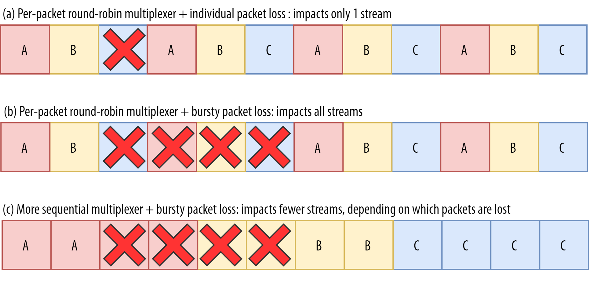
To lower the risk of multiple streams being affected by a lossy burst, we need to concatenate more data for each stream. For example, AABBCCAABBCCAABBCCAABBCC… is a small improvement, and AAAABBBBCCCCAAAABBBBCCCC… (see bottom row in figure 8 above) is even better. You can again see that a more sequential approach is better, even though that reduces the chances that we have multiple concurrent active streams.
In the end, predicting the actual impact of QUIC’s HoL blocking removal is difficult, because it depends on the number of streams, the size and frequency of the loss bursts, how the stream data is actually used, etc. However, most results at this time indicate it will not help much for the use case of web-page loading, because there we typically want fewer concurrent streams.
If you want even more detail on this topic or just some concrete examples, please check out my in-depth article on HTTP HoL blocking.
Did You Know?
As with the previous sections, some advanced techniques can help us here. For example, modern congestion controllers use packet pacing. This means that they don’t send, for example, 100 packets in a single burst, but rather spread them out over an entire RTT. This conceptually lowers the chances of overloading the network, and the QUIC Recovery RFC strongly recommends using it. Complementarily, some congestion-control algorithms such as BBR don’t keep increasing their send rate until they cause packet loss, but rather back off before that (by looking at, for example, RTT fluctuations, because RTTs also rise when a network is becoming overloaded).
While these approaches lower the overall chances of packet loss, they don’t necessarily lower its burstiness.
What does it all mean?
While QUIC’s HoL blocking removal means, in theory, that it (and HTTP/3) should perform better on lossy networks, in practice this depends on a lot of factors. Because the use case of web-page loading typically favours a more sequential multiplexing set-up, and because packet loss is unpredictable, this feature would, again, likely affect mainly the slowest 1% of users. However, this is still a very active area of research, and only time will tell.
Still, there are situations that might see more improvements. These are mostly outside of the typical use case of the first full page load — for example, when resources are not render blocking, when they can be processed incrementally, when streams are completely independent, or when less data is sent at the same time.
Examples include repeat visits on well-cached pages and background downloads and API calls in single-page apps. For example, Facebook has seen some benefits from HoL blocking removal when using HTTP/3 to load data in its native app.
UDP and TLS Performance
A fifth performance aspect of QUIC and HTTP/3 is about how efficiently and performantly they can actually create and send packets on the network. We will see that QUIC’s usage of UDP and heavy encryption can make it a fair bit slower than TCP (but things are improving).
First, we’ve already discussed that QUIC’s usage of UDP was more about flexibility and deployability than about performance. This is evidenced even more by the fact that, up until recently, sending QUIC packets over UDP was typically much slower than sending TCP packets. This is partly because of where and how these protocols are typically implemented (see figure 9 below).
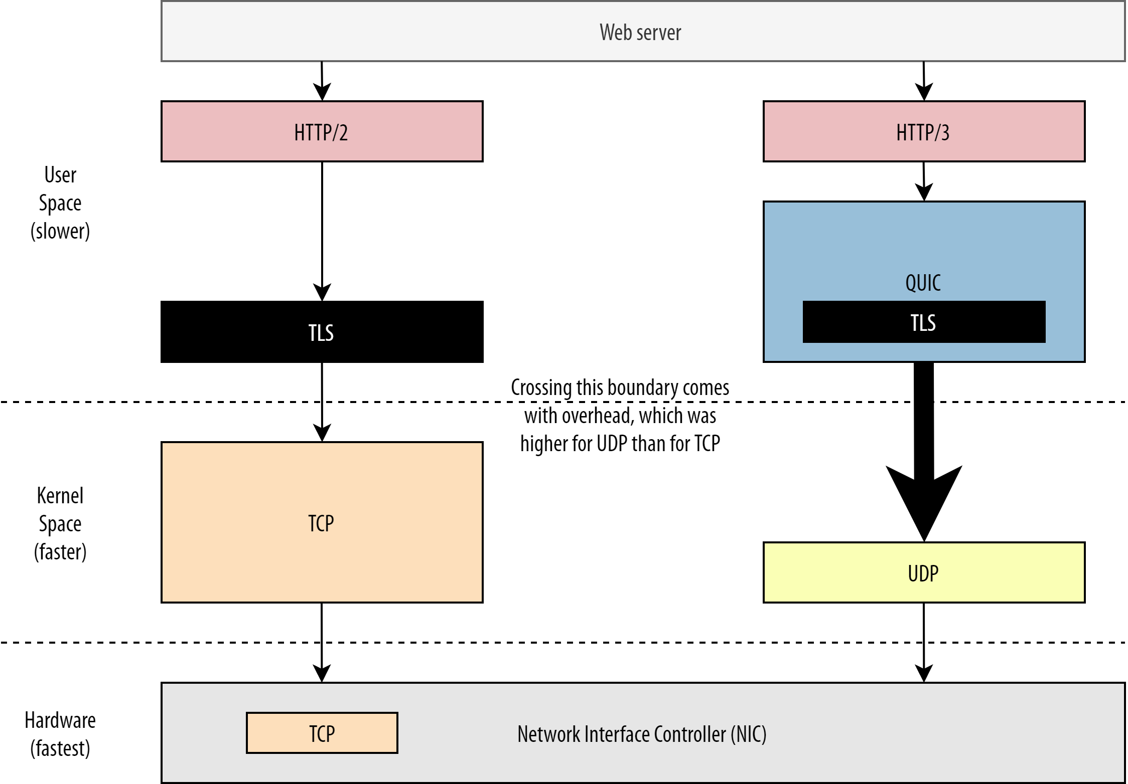
As discussed above, TCP and UDP are typically implemented directly in the OS’ fast kernel. In contrast, TLS and QUIC implementations are mostly in slower user space (note that this is not really needed for QUIC — it is mostly done because it’s much more flexible). This makes QUIC already a bit slower than TCP.
Additionally, when sending data from our user-space software (say, browsers and web servers), we need to pass this data to the OS kernel, which then uses TCP or UDP to actually put it on the network. Passing this data is done using kernel APIs (system calls), which involves a certain amount of overhead per API call. For TCP, these overheads were much lower than for UDP.
This is mostly because, historically, TCP has been used a lot more than UDP. As such, over time, many optimizations were added to TCP implementations and kernel APIs to reduce packet send and receive overheads to a minimum. Many network interface controllers (NICs) even have built-in hardware-offload features for TCP. UDP, however, was not as lucky, because its more limited use didn’t justify the investment in added optimizations. In the past five years, this has luckily changed, and most OSes have since added optimized options for UDP as well.
Secondly, QUIC has a lot of overhead because it encrypts each packet individually. This is slower than using TLS over TCP, because there you can encrypt packets in chunks (up to about 16 KB or 11 packets at a time), which is more efficient. This was a conscious trade-off made in QUIC, because bulk encryption can lead to its own forms of HoL blocking.
Unlike the first point, where we could add extra APIs to make UDP (and thus QUIC) faster, here, QUIC will always have an inherent disadvantage to TCP + TLS. However, this is also quite manageable in practice with, for example, optimized encryption libraries and clever methods that allow QUIC packets headers to be encrypted in bulk.
As a result, while Google’s earliest QUIC versions were still twice as slow as TCP + TLS, things have certainly improved since. For example, in recent tests, Microsoft’s heavily optimized QUIC stack was able to get 7.85 Gbps, compared to 11.85 Gbps for TCP + TLS on the same system (so here, QUIC is about 66% as fast as TCP + TLS).
This is with the recent Windows updates, which made UDP faster (for a full comparison, UDP throughput on that system was 19.5 Gbps). The most optimized version of Google’s QUIC stack is currently about 20% slower than TCP + TLS. Earlier tests by Fastly on a less advanced system and with a few tricks even claim equal performance (about 450 Mbps), showing that depending on the use case, QUIC can definitely compete with TCP.
However, even if QUIC were twice as slow as TCP + TLS, it’s not all that bad. First, QUIC and TCP + TLS processing is typically not the heaviest thing happening on a server, because other logic (say, HTTP, caching, proxying, etc.) also needs to execute. As such, you won’t actually need twice as many servers to run QUIC (it’s a bit unclear how much impact it will have in a real data center, though, because none of the big companies have released data on this).
Secondly, there are still plenty of opportunities to optimize QUIC implementations in the future. For example, over time, some QUIC implementations will (partially) move to the OS kernel (much like TCP) or bypass it (some already do, like MsQuic and Quant). We can also expect QUIC-specific hardware to become available.
Still, there will likely be some use cases for which TCP + TLS will remain the preferred option. For example, Netflix has indicated that it probably won’t move to QUIC anytime soon, having heavily invested in custom FreeBSD set-ups to stream its videos over TCP + TLS.
Similarly, Facebook has said that QUIC will probably mainly be used between end users and the CDN’s edge, but not between data centers or between edge nodes and origin servers, due to its larger overhead. In general, very high-bandwidth scenarios will probably continue to favour TCP + TLS, especially in the next few years.
Did You Know?
Optimizing network stacks is a deep and technical rabbit hole of which the above merely scratches the surface (and misses a lot of nuance). If you’re brave enough or if you want to know what terms like GRO/GSO, SO_TXTIME, kernel bypass, and sendmmsg() and recvmmsg() mean, I can recommend some excellent articles on optimizing QUIC by Cloudflare and Fastly, as well as an extensive code walkthrough by Microsoft, and an in-depth talk from Cisco. Finally, a Google engineer gave a very interesting keynote about optimizing their QUIC implementation over time.
What does it all mean?
QUIC’s particular usage of the UDP and TLS protocols has historically made it much slower than TCP + TLS. However, over time, several improvements have been made (and will continue to be implemented) that have closed the gap somewhat. You probably won’t notice these discrepancies in typical use cases of web-page loading, though, but they might give you headaches if you maintain large server farms.
HTTP/3 Features
Up until now, we’ve mainly talked about new performance features in QUIC versus TCP. However, what about HTTP/3 versus HTTP/2? As discussed in part 1, HTTP/3 is really HTTP/2-over-QUIC, and as such, no real, big new features were introduced in the new version. This is unlike the move from HTTP/1.1 to HTTP/2, which was much larger and introduced new features such as header compression, stream prioritization, and server push. These features are all still in HTTP/3, but there are some important differences in how they are implemented under the hood.
This is mostly because of how QUIC’s removal of HoL blocking works. As we’ve discussed, a loss on stream B no longer implies that streams A and C will have to wait for B’s retransmissions, like they did over TCP. As such, if A, B, and C each sent a QUIC packet in that order, their data might well be delivered to (and processed by) the browser as A, C, B! Put differently, unlike TCP, QUIC is no longer fully ordered across different streams!
This is a problem for HTTP/2, which really relied on TCP’s strict ordering in the design of many of its features, which use special control messages interspersed with data chunks. In QUIC, these control messages might arrive (and be applied) in any order, potentially even making the features do the opposite of what was intended! The technical details are, again, unnecessary for this article, but the first half of this paper should give you an idea of how stupidly complex this can get.
As such, the internal mechanics and implementations of the features have had to change for HTTP/3. A concrete example is HTTP header compression, which lowers the overhead of repeated large HTTP headers (for example, cookies and user-agent strings). In HTTP/2, this was done using the HPACK set-up, while for HTTP/3 this has been reworked to the more complex QPACK. Both systems deliver the same feature (i.e. header compression) but in quite different ways. Some excellent deep technical discussion and diagrams on this topic can be found on the Litespeed blog.
Something similar is true for the prioritization feature that drives stream multiplexing logic and which we’ve briefly discussed above. In HTTP/2, this was implemented using a complex “dependency tree” set-up, which explicitly tried to model all page resources and their interrelations (more information is in the talk “The Ultimate Guide to HTTP Resource Prioritization”). Using this system directly over QUIC would lead to some potentially very wrong tree layouts, because adding each resource to the tree would be a separate control message.
Additionally, this approach turned out to be needlessly complex, leading to many implementation bugs and inefficiencies and subpar performance on many servers. Both problems have led the prioritization system to be redesigned for HTTP/3 in a much simpler way. This more straightforward set-up makes some advanced scenarios difficult or impossible to enforce (for example, proxying traffic from multiple clients on a single connection), but still enables a wide range of options for web-page loading optimization.
While, again, the two approaches deliver the same basic feature (guiding stream multiplexing), the hope is that HTTP/3’s easier set-up will make for fewer implementation bugs.
Finally, there is server push. This feature allows the server to send HTTP responses without waiting for an explicit request for them first. In theory, this could deliver excellent performance gains. In practice, however, it turned out to be hard to use correctly and inconsistently implemented. As a result, it is probably even going to be removed from Google Chrome.
Despite all this, it _is_ still defined as a feature in HTTP/3 (although few implementations support it). While its internal workings haven’t changed as much as the previous two features, it too has been adapted to work around QUIC’s non-deterministic ordering. Sadly, though, this will do little to solve some of its longstanding issues.
What does it all mean?
As we’ve said before, most of HTTP/3’s potential comes from the underlying QUIC, not HTTP/3 itself. While the protocol’s internal implementation is very different from HTTP/2’s, its high-level performance features and how they can and should be used have stayed the same.
Future Developments to Look Out For
In this series, I have regularly highlighted that faster evolution and higher flexibility are core aspects of QUIC (and, by extension, HTTP/3). As such, it should be no surprise that people are already working on new extensions to and applications of the protocols. Listed below are the main ones that you’ll probably encounter somewhere down the line:
Forward error correction
This purpose of this technique is, again, to improve QUIC’s resilience to packet loss. It does this by sending redundant copies of the data (though cleverly encoded and compressed so that they’re not as large). Then, if a packet is lost but the redundant data arrives, a retransmission is no longer needed.
This was originally a part of Google QUIC (and one of the reasons why people say QUIC is good against packet loss), but it is not included in the standardized QUIC version 1 because its performance impact wasn’t proven yet. Researchers are now performing active experiments with it, though, and you can help them out by using the PQUIC-FEC Download Experiments app.
Multipath QUIC
We’ve previously discussed connection migration and how it can help when moving from, say, Wi-Fi to cellular. However, doesn’t that also imply we might use both Wi-Fi and cellular at the same time? Concurrently using both networks would give us more available bandwidth and increased robustness! That is the main concept behind multipath.
This is, again, something that Google experimented with but that didn’t make it into QUIC version 1 due to its inherent complexity. However, researchers have since shown its high potential, and it might make it into QUIC version 2. Note that TCP multipath also exists, but that has taken almost a decade to become practically usable.
Unreliable data over QUIC and HTTP/3
As we’ve seen, QUIC is a fully reliable protocol. However, because it runs over UDP, which is unreliable, we can add a feature to QUIC to also send unreliable data. This is outlined in the proposed datagram extension. You would, of course, not want to use this to send web page resources, but it might be handy for things such as gaming and live video streaming. This way, users would get all of the benefits of UDP but with QUIC-level encryption and (optional) congestion control.
WebTransport
Browsers don’t expose TCP or UDP to JavaScript directly, mainly due to security concerns. Instead, we have to rely on HTTP-level APIs such as Fetch and the somewhat more flexible WebSocket and WebRTC protocols. The newest in this series of options is called WebTransport, which mainly allows you to use HTTP/3 (and, by extension, QUIC) in a more low-level way (although it can also fall back to TCP and HTTP/2 if needed).
Crucially, it will include the ability to use unreliable data over HTTP/3 (see the previous point), which should make things such as gaming quite a bit easier to implement in the browser. For normal (JSON) API calls, you’ll, of course, still use Fetch, which will also automatically employ HTTP/3 when possible. WebTransport is still under heavy discussion at the moment, so it’s not yet clear what it will eventually look like. Of the browsers, only Chromium is currently working on a public proof-of-concept implementation.
DASH and HLS video streaming
For non-live video (think YouTube and Netflix), browsers typically make use of the Dynamic Adaptive Streaming over HTTP (DASH) or HTTP Live Streaming (HLS) protocols. Both basically mean that you encode your videos into smaller chunks (of 2 to 10 seconds) and different quality levels (720p, 1080p, 4K, etc.).
At runtime, the browser estimates the highest quality your network can handle (or the most optimal for a given use case), and it requests the relevant files from the server via HTTP. Because the browser doesn’t have direct access to the TCP stack (as that’s typically implemented in the kernel), it occasionally makes a few mistakes in these estimates, or it takes a while to react to changing network conditions (leading to video stalls).
Because QUIC is implemented as part of the browser, this could be improved quite a bit, by giving the streaming estimators access to low-level protocol information (such as loss rates, bandwidth estimates, etc.). Other researchers have been experimenting with mixing reliable and unreliable data for video streaming as well, with some promising results.
Protocols other than HTTP/3
With QUIC being a general purpose transport protocol, we can expect many application-layer protocols that now run over TCP to be run on top of QUIC as well. Some works in progress include DNS-over-QUIC, SMB-over-QUIC, and even SSH-over-QUIC. Because these protocols typically have very different requirements than HTTP and web-page loading, QUIC’s performance improvements that we’ve discussed might work much better for these protocols.
What does it all mean?
QUIC version 1 is just the start. Many advanced performance-oriented features that Google had earlier experimented with did not make it into this first iteration. However, the goal is to quickly evolve the protocol, introducing new extensions and features at a high frequency. As such, over time, QUIC (and HTTP/3) should become clearly faster and more flexible than TCP (and HTTP/2).
Conclusion
In this second part of the series, we have discussed the many different performance features and aspects of HTTP/3 and especially QUIC. We have seen that while most of these features seem very impactful, in practice they might not do all that much for the average user in the use case of web-page loading that we’ve been considering.
For example, we’ve seen that QUIC’s use of UDP doesn’t mean that it can suddenly use more bandwidth than TCP, nor does it mean that it can download your resources more quickly. The often-lauded 0-RTT feature is really a micro-optimization that saves you one round trip, in which you can send about 5 KB (in the worst case).
HoL blocking removal doesn’t work well if there is bursty packet loss or when you’re loading render-blocking resources. Connection migration is highly situational, and HTTP/3 doesn’t have any major new features that could make it faster than HTTP/2.
As such, you might expect me to recommend that you just skip HTTP/3 and QUIC. Why bother, right? However, I will most definitely do no such thing! Even though these new protocols might not aid users on fast (urban) networks much, the new features do certainly have the potential to be highly impactful to highly mobile users and people on slow networks.
Even in Western markets such as my own Belgium, where we generally have fast devices and access to high-speed cellular networks, these situations can affect 1% to even 10% of your user base, depending on your product. An example is someone on a train trying desperately to look up a critical piece of information on your website, but having to wait 45 seconds for it to load. I certainly know I’ve been in that situation, wishing someone had deployed QUIC to get me out of it.
However, there are other countries and regions where things are much worse still. There, the average user might look a lot more like the slowest 10% in Belgium, and the slowest 1% might never get to see a loaded page at all. In many parts of the world, web performance is an accessibility and inclusivity problem.
This is why we should never just test our pages on our own hardware (but also use a service like Webpagetest) and also why you should definitely deploy QUIC and HTTP/3. Especially if your users are often on the move or unlikely to have access to fast cellular networks, these new protocols might make a world of difference, even if you don’t notice much on your cabled MacBook Pro. For more details, I highly recommend Fastly’s post on the issue.
If that doesn’t fully convince you, then consider that QUIC and HTTP/3 will continue to evolve and get faster in the years to come. Getting some early experience with the protocols will pay off down the road, allowing you to reap the benefits of new features as soon as possible. Additionally, QUIC enforces security and privacy best practices in the background, which benefit all users everywhere.
Finally convinced? Then stay tuned for part 3 of the series to read about how you can go about using the new protocols in practice.
This series is divided into three parts:
HTTP/3 history and core concepts
This is targeted at people new to HTTP/3 and protocols in general, and it mainly discusses the basics. HTTP/3 performance features (current article)
This is more in depth and technical. People who already know the basics can start here. Practical HTTP/3 deployment options (coming up soon!)
This explains the challenges involved in deploying and testing HTTP/3 yourself. It details how and if you should change your web pages and resources as well.